Elastic Analysis
CalcpadCE provides closed-form analytical solutions for classical elastic problems — useful as benchmarks for validating finite-element models, for fast parametric studies before committing to a mesh, and as hand-check baselines on engineering reports.
The three worksheets below all hinge on Fourier series expansions of the loading or compatibility conditions, with the number of retained terms exposed as an input. The deep-beam stress field follows Filonenko-Borodich's plane-stress series solution; the rectangular slab uses the Navier double-trigonometric series from Kirchhoff–Love plate theory; and the rectangular-section Saint-Venant torsion recovers the warping shear-stress field from a single sine series.
Every geometric and material input is parametric, so each worksheet doubles as a sensitivity tool: change the slab aspect ratio, the load span on the deep beam, or the cross-section proportions for torsion and the report — equations, numbers and plots — updates in one pass.
Deep Beam
Plane-stress analysis of a simply-supported deep beam under a partial uniform load, using a sine-series decomposition of the load and reaction. Recovers \(σ_x\), \(σ_y\) and \(τ_{xy}\) for arbitrary length, height, load span and support width — an analytical baseline for FE checks.
#rad
'<h3>Input data</h3>
'<table><tr><td>
'Beam length -'l = ? {4}m
'Height -'h = ? {2}m
'Load -'q = ? {100}*(kN/m)
'Length of load -'b = ? {0.8}m
'Distance to load start -'a = ? {1.6}m
'Length of support -'d = ? {0.4}m
'Number of iterations -'N = ? {21}
'</td><td><img src="../../Images/mechanics/elastic/deep-beam-fea.png" style="height:160pt; width:150pt; margin-left:50pt;"></td></tr></table>
#hide
c = a + b
q(x) = if((x < a) + (x > c); 0kN/m; q)
α(n) = n*π/l
αh(n) = n*π*h/l
q_n(n) = 2*q/(α(n)*l)*(cos(α(n)*a) - cos(α(n)*c))
r = q*b/(2*d)
e = l - d
r(x) = if((x < d) + (x > e); r; 0kN/m)
r_n(n) = 2*r/(α(n)*l)*(1 - cos(α(n)*l) - (cos(α(n)*d) - cos(α(n)*e)))
q_series(x) = $Sum{q_n(n)*sin(α(n)*x) @ n = 1 : N}
r_series(x) = $Sum{r_n(n)*sin(α(n)*x) @ n = 1 : N}
PlotWidth = 400
PlotHeight = 150
#post
'Original and Fourier functions for the load
$Plot{q(x) & q_series(x) @ x = 0m : l}
'Original and Fourier functions for the reaction in supports
$Plot{r(x) & r_series(x) @ x = 0m : l}
#hide
sh(n) = sinh(αh(n))
cth(n) = coth(αh(n))
β(n) = αh(n)/sh(n)
Δ(n) = α(n)*(1 - β(n))*(1 + β(n))
A(n) = r_n(n)/α(n)^2
B(n) = q_n(n)*(1/sh(n) + β(n)*cth(n))/(α(n)*Δ(n)) - r_n(n)*(cth(n) + β(n)/sh(n))/(α(n)*Δ(n))
C(n) = -B(n)*α(n)
D(n) = (q_n(n)*β(n) - r_n(n))/Δ(n)
ch(n; x) = cosh(α(n)*x)
th(n; x) = tanh(α(n)*x)
Y(n; y) = ch(n; y)*(A(n) + B(n)*th(n; y) + C(n)*y + D(n)*y*th(n; y))
Y_1(n; y) = ch(n; y)*(α(n)*(A(n)*th(n; y) + B(n)) + C(n)*(1 + α(n)*y*th(n; y)) + D(n)*(th(n; y) + α(n)*y))
Y_2(n; y) = ch(n; y)*α(n)*(A(n)*α(n) + B(n)*α(n)*th(n; y) + C(n)*(2*th(n; y) + α(n)*y) + D(n)*(2 + α(n)*y*th(n; y)))
Y(N; 0m) - r_n(N)/α(N)^2
Y_1(N; 0m)
Y_1(N; h)
Y(N; h) - q_n(N)/α(N)^2
PlotStep = 5
PlotHeight = PlotWidth*h/l
#post
'<h3>Calculation of stresses</h3>
σ_x(x; y) = $Sum{Y_2(n; y)*sin(α(n)*x) @ n = 1 : N}
'<!--'k = round(abs(σ_x(l/2; h))/20)*50'-->
$Map{σ_x(x; y) @ x = 0m : l & y = 0m : h}
'Plot for σ<sub>x</sub> at <var>x</var> = <var>l</var>/2
$Plot{σ_x(l/2; y)|y & -k|0m & k|0m @ y = 0m : h}
'Bottom value -'σ_x(l/2; 0m)
'Top value -'σ_x(l/2; h)
σ_y(x; y) = -$Sum{α(n)^2*Y(n; y)*sin(α(n)*x) @ n = 1 : N}
$Map{σ_y(x; y) @ x = 0m : l & y = 0m : h}
'Top value -'σ_y(l/2; h)
τ_xy(x; y) = -$Sum{α(n)*Y_1(n; y)*cos(α(n)*x) @ n = 1 : N}
$Map{τ_xy(x; y) @ x = 0m : l & y = 0m : h}
'Value at 3/4 of span -'τ_xy(3*l/4; h/2)
σ_m(x; y) = 0.5*(σ_x(x; y) + σ_y(x; y))
Δσ(x; y) = 0.5*sqr((σ_x(x; y) - σ_y(x; y))^2 + 4*τ_xy(x; y)^2)
σ_1(x; y) = σ_m(x; y) + Δσ(x; y)
$Map{σ_1(x; y) @ x = 0m : l & y = 0m : h}
σ_2(x; y) = σ_m(x; y) - Δσ(x; y)
$Map{σ_2(x; y) @ x = 0m : l & y = 0m : h}
|
Beam length - l = 4 m Height - h = 2 m Load - q = 100 kNm Length of load - b = 0.8 m Distance to load start - a = 1.6 m Length of support - d = 0.4 m Number of iterations - N = 21 | 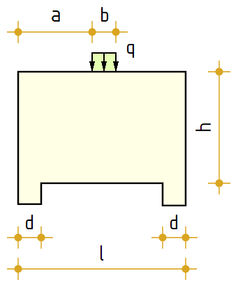 |
Original and Fourier functions for the load

Original and Fourier functions for the reaction in supports

σx ( x; y ) = N∑n= 1Y2 ( n; y ) · sin ( α ( n ) · x )

Plot for σx at x = l/2

Bottom value - σx (l2; 0 m) = σx (4 m2; 0 m) = 95.66 kN ∕ m
Top value - σx (l2; h) = σx (4 m2; 2 m) = -147.56 kN ∕ m
σy ( x; y ) = -N∑n= 1α ( n ) 2 · Y ( n; y ) · sin ( α ( n ) · x )

Top value - σy (l2; h) = σy (4 m2; 2 m) = -92.32 kN ∕ m
τxy ( x; y ) = -N∑n= 1α ( n ) · Y1 ( n; y ) · cos ( α ( n ) · x )

Value at 3/4 of span - τxy (3 · l4; h2) = τxy (3 · 4 m4; 2 m2) = 29.96 kN ∕ m
σm ( x; y ) = 0.5 · ( σx ( x; y ) + σy ( x; y ) )
Δσ ( x; y ) = 0.5 · √ ( σx ( x; y ) − σy ( x; y ) ) 2 + 4 · τxy ( x; y ) 2
σ1 ( x; y ) = σm ( x; y ) + Δσ ( x; y )

σ2 ( x; y ) = σm ( x; y ) − Δσ ( x; y )

Rectangular Slab
Navier double-trig-series solution for a thin rectangular plate on simple supports under uniform load. Returns maximum deflection and bending moments \(M_x\), \(M_y\) for arbitrary plan dimensions, thickness and elastic constants — a quick parametric check against slab FEA.
'<h3>Input data</h3>
'Dimensions in plan -'a = ? {6}m','b = ? {4}m
'<table><tr><td>
'Slab thickness -'t = ? {0.1}m
'Distributed load -'q = ? {10}*(kN/m^2)
'Elastic modulus -'E = ? {35000}MPa
'Poisson`s ratio -'ν = ? {0.15}
'Number of iterations -'N = ? {5}
'</td><td><img src="../../Images/mechanics/elastic/slab.png" style="height:110pt; width:145pt; margin-left:40pt;"></td></tr></table>
#rad
#post
'<h3>Analysis</h3>
'Cylindrical stiffness -'D = E*t^3/(12*(1 - ν^2))
α = a/b
α_2 = α^2
q_0 = 16*q/π^2
'Auxiliary functions
k(n) = 2*n + 1
k_2(n) = 4*n*(n + 1) + 1
A(m; n) = k_2(m) + α_2*k_2(n)' => 'A_1(m; n) = 1/A(m; n)^2
B(m; n) = k_2(m) + ν*α_2*k_2(n)' => 'B_1(m; n) = B(m; n)/A(m; n)^2
C(m; n) = ν*k_2(m) + α_2*k_2(n)' => 'C_1(m; n) = C(m; n)/A(m; n)^2
S_a(m; x) = sin(k(m)*π/a*x)/k(m)', 'S_b(n; y) = sin(k(n)*π/b*y)/k(n)
#hide
PlotWidth = 50*a
PlotHeight = 50*b
PlotStep = 10
#post
'Deflections
w(x; y) = q_0*(a/π)^4/D*$Sum{S_a(m; x)*$Sum{A_1(m; n)*S_b(n; y) @ n = 0 : N} @ m = 0 : N}|mm
'Bending moments
M_x(x; y) = q_0*(a/π)^2*$Sum{S_a(m; x)*$Sum{B_1(m; n)*S_b(n; y) @ n = 0 : N} @ m = 0 : N}
M_y(x; y) = q_0*(a/π)^2*$Sum{S_a(m; x)*$Sum{C_1(m; n)*S_b(n; y) @ n = 0 : N} @ m = 0 : N}
k_1(n) = 2*n
M_xy(x; y) = -q_0*((a/π)^2)*(1 - ν)*α*$Sum{cos(k(m)*π*x/a)*$Sum{A_1(m; n)*cos(k(n)*π*y/b) @ n = 0 : N} @ m = 0 : N}
'Principal bending moments
M_max(x; y) = (M_x(x; y) + M_y(x; y))/2 + sqrt((M_x(x; y) - M_y(x; y))^2/4 + M_xy(x; y)^2)
M_min(x; y) = (M_x(x; y) + M_y(x; y))/2 - sqrt((M_x(x; y) - M_y(x; y))^2/4 + M_xy(x; y)^2)
'<h3>Results</h3>
'Deflections
$Map{-w(x; y) @ x = 0m : a & y = 0m : b}
'Maximum value -'w(a/2; b/2)
'Bending moments - Mx, kNm/m
$Map{M_x(x; y) @ x = 0m : a & y = 0m : b}
'Maximum value -'M_x(a/2; b/2)|kNm/m
'Bending moments - My, kNm/m
$Map{M_y(x; y) @ x = 0m : a & y = 0m : b}
'Maximum value -'M_y(a/2; b/2)|kNm/m
'Bending moments - Mxy, kNm/m
$Map{M_xy(x; y) @ x = 0m : a & y = 0m : b}
'Maximum value -'M_xy(0m; 0m)|kNm/m
'Principal bending moments - Mmax, kNm/m
$Map{M_min(x; y) @ x = 0m : a & y = 0m : b}
'Maximum value -'M_max(a/2; b/2)|kNm/m
'Principal bending moments - Mmin, kNm/m
$Map{M_min(x; y) @ x = 0m : a & y = 0m : b}
'Maximum value -'M_min(b/2; b/2)|kNm/m
'Minimum value -'M_min(0m; 0m)|kNm/m
Dimensions in plan - a = 6 m , b = 4 m
|
Slab thickness - t = 0.1 m Distributed load - q = 10 kNm2 Elastic modulus - E = 35000 MPa Poisson`s ratio - ν = 0.15 Number of iterations - N = 5 | 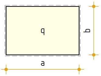 |
Cylindrical stiffness - D = E · t312 · ( 1 − ν2 ) = 35000 MPa · ( 0.1 m ) 312 · ( 1 − 0.152 ) = 2983.8 kNm
α = ab = 6 m4 m = 1.5
α2 = α2 = 1.52 = 2.25
q0 = 16 · qπ2 = 16 · 10 kN ∕ m23.142 = 16.21 kN ∕ m2
Auxiliary functions
k ( n ) = 2 · n + 1
k2 ( n ) = 4 · n · ( n + 1 ) + 1
A ( m; n ) = k2 ( m ) + α2 · k2 ( n ) => A1 ( m; n ) = 1A ( m; n ) 2
B ( m; n ) = k2 ( m ) + ν · α2 · k2 ( n ) => B1 ( m; n ) = B ( m; n ) A ( m; n ) 2
C ( m; n ) = ν · k2 ( m ) + α2 · k2 ( n ) => C1 ( m; n ) = C ( m; n ) A ( m; n ) 2
Sa ( m; x ) = sin(k ( m ) · πa · x)k ( m ) , Sb ( n; y ) = sin(k ( n ) · πb · y)k ( n )
Deflections
w ( x; y ) = q0 · (aπ)4D · N∑m= 0Sa ( m; x ) · N∑n= 0A1 ( m; n ) · Sb ( n; y )
Bending moments
Mx ( x; y ) = q0 · (aπ)2 · N∑m= 0Sa ( m; x ) · N∑n= 0B1 ( m; n ) · Sb ( n; y )
My ( x; y ) = q0 · (aπ)2 · N∑m= 0Sa ( m; x ) · N∑n= 0C1 ( m; n ) · Sb ( n; y )
k1 ( n ) = 2 · n
Mxy ( x; y ) = -q0 · (aπ)2 · ( 1 − ν ) · α · N∑m= 0cos(k ( m ) · π · xa) · N∑n= 0A1 ( m; n ) · cos(k ( n ) · π · yb)
Principal bending moments
Mmax ( x; y ) = Mx ( x; y ) + My ( x; y ) 2 + ( Mx ( x; y ) − My ( x; y ) ) 24 + Mxy ( x; y ) 2
Mmin ( x; y ) = Mx ( x; y ) + My ( x; y ) 2 − ( Mx ( x; y ) − My ( x; y ) ) 24 + Mxy ( x; y ) 2
Deflections

Maximum value - w (a2; b2) = w (6 m2; 4 m2) = 6.63 mm
Bending moments - Mx, kNm/m

Maximum value - Mx (a2; b2) = Mx (6 m2; 4 m2) = 6.22 kNm ∕ m
Bending moments - My, kNm/m

Maximum value - My (a2; b2) = My (6 m2; 4 m2) = 12.31 kNm ∕ m
Bending moments - Mxy, kNm/m

Maximum value - Mxy ( 0 m; 0 m ) = -8.3 kNm ∕ m
Principal bending moments - Mmax, kNm/m

Maximum value - Mmax (a2; b2) = Mmax (6 m2; 4 m2) = 12.31 kNm ∕ m
Principal bending moments - Mmin, kNm/m
Maximum value - Mmin (b2; b2) = Mmin (4 m2; 4 m2) = 6.13 kNm ∕ m
Minimum value - Mmin ( 0 m; 0 m ) = -8.3 kNm ∕ m
Saint-Venant Torsion
Closed-form Saint-Venant torsion of a rectangular cross-section, evaluating the shear-stress field \(τ_{zx}\), \(τ_{zy}\) and torsional rigidity from a single Fourier series. A hand-check baseline for FE torsion models and for simplified rectangular-section design formulas.
'<h3>Input data</h3>
'<table><tr><td>
'Dimensions of cross section
a = ? {50}cm','b = ? {30}*(cm/2)
'Torsional moment -'M_t = ? {20}kNm
'Number of iterations -'n = ? {10}
'</td><td><img src="../../Images/mechanics/elastic/torsion.png" style="height:110pt; width:152pt; margin-left:50pt;"></td></tr></table>
#post
'<h3>Analysis</h3>
k(i) = 2*i + 1', 'α(i) = k(i)*π/a
#hide
#rad
c = 400/a
PlotWidth = a*c
PlotHeight = 2*b*c
PlotStep = 10
#post
'Factors for calculation
C = M_t/(4*a^4*(b/(12*a) - 8/π^5*$Sum{1/k(i)^5*tanh(α(i)*b) @ i = 0 : n}))|MPa/m
C_1 = 4*C*a/π^2|MPa
'Shear stress calculation
τ_zx(x; y) = C_1*$Sum{1/(k(i)^2*cosh(α(i)*b))*sinh(α(i)*y)*sin(α(i)*x) @ i = 0 : n}|MPa
τ_zy(x; y) = C*(a/2 - x) - C_1*$Sum{1/(k(i)^2*cosh(α(i)*b))*cosh(α(i)*y)*cos(α(i)*x) @ i = 0 : n}|MPa
'<h3>Results</h3>
'Peak values
τ_zx(a/2; b)
τ_zy(0cm; 0cm)
'Stress surface plots
'τ_zx
$Map{τ_zx(x; y) @ x = 0cm : a & y = -b : b}
'τ_zy
$Map{τ_zy(x; y) @ x = 0cm : a & y = -b : b}
#hide
c = 0.25*b/τ_zx(a/2; b)|cm/kPa
x(k) = k*a
y(k) = (2*k - 1)*b
#post
'Stress line plots
$Plot{a/2 + c*τ_zx(a/2; y(k))|y(k) & a/2|y(k) & x(k)|0cm & a + c*τ_zy(a; y(k))|y(k) & x(k)|c*τ_zy(x(k); 0cm) & x(k)|b - c*τ_zx(x(k); b) @ k = 0 : 1}
|
Dimensions of cross section a = 50 cm , b = 30 · cm2 = 15 cm Torsional moment - Mt = 20 kNm Number of iterations - n = 10 | 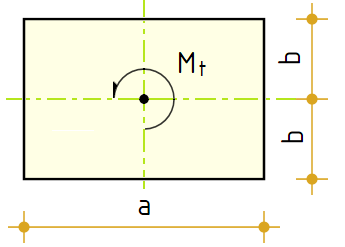 |
k ( i ) = 2 · i + 1 , α ( i ) = k ( i ) · πa
Factors for calculation
C = Mt4 · a4 · (b12 · a − 8π5 · n∑i= 01k ( i ) 5 · tanh ( α ( i ) · b ) ) = 20 kNm4 · ( 50 cm ) 4 · (15 cm12 · 50 cm − 83.145 · 0.741) = 14.2 MPa ∕ m
C1 = 4 · C · aπ2 = 4 · 14.2 MPa ∕ m · 50 cm3.142 = 2.88 MPa
Shear stress calculation
τzx ( x; y ) = C1 · n∑i= 01k ( i ) 2 · cosh ( α ( i ) · b ) · sinh ( α ( i ) · y ) · sin ( α ( i ) · x )
τzy ( x; y ) = C · (a2 − x) − C1 · n∑i= 01k ( i ) 2 · cosh ( α ( i ) · b ) · cosh ( α ( i ) · y ) · cos ( α ( i ) · x )
Peak values
τzx (a2; b) = τzx (50 cm2; 15 cm) = 1.88 MPa
τzy ( 0 cm; 0 cm ) = 1.56 MPa
Stress surface plots
τ_zx

τ_zy

Stress line plots

Spotted an error? Edit these examples.