Nonlinear

CalcpadCE worksheets in this section present geometrically nonlinear truss analysis, where the equilibrium equations are written in the deformed configuration so that large displacements and snap-through behaviour are captured naturally. The system of equations is implicit in the joint displacements and is therefore solved iteratively — by fixed-point iteration, Newton-Raphson, the secant method, and the built-in Root solver based on a modified Anderson-Björck bracketing scheme.

A symmetric two-bar Biot truss demonstrates the four numerical methods on a system that is linearly unstable: the equilibrium has to be derived for the deformed length \(l'(v) = \sqrt{(l + u)^2 + v^2}\) and the vertical reaction \(F_y(v) = E A \cdot \Delta l(v) / l \cdot v / l'(v)\) is then balanced against the applied load. A shallow Von-Mises truss extends the same formulation to a tube section with a small initial rise, where the load-displacement curve passes through a limit point and the post-buckling branch is followed. A prestressed asymmetric Biot truss combines geometric nonlinearity with a bilinear elastic-plastic material law, so that the element stiffness \(E A\) switches from \(E_0 A\) to \(E_1 A\) once the strain exceeds the yield value \(\varepsilon_y\), and a global Newton-Raphson loop updates the Jacobi matrix at each iteration.

A small SVG drawing library, svg_drawing.cpd, is included by each worksheet to render the undeformed and deformed configurations, supports and applied forces directly into the report.

Material and Geometric Nonlinear Analysis of Prestressed Asymmetric Biot Truss

Combined material and geometric nonlinear analysis of a prestressed three-joint truss with a bilinear elastic-plastic stress-strain law, solved by a global Newton-Raphson iteration that updates the Jacobi matrix and the axial stiffness \(E A\) at each step.

Code:

'<h4>Input data</h4>
#deg
#hide
δz = 10^-12
Precision = 10^-9
x_J = [0; 3; 9]*m
y_J = [0; 0; 0]*m
#show
x_J','y_J', 'n_J = len(x_J)
'<h4>Elements - [J1; J2]</h4>
#hide
E_J = [1; 2|2; 3]
#show
transp(E_J)', 'n_E = n_rows(E_J)', 'J_1(e) = E_J.(e; 1)', 'J_2(e) = E_J.(e; 2)
'Element endpoint coordinates
x_1(e) = x_J.J_1(e)','y_1(e) = y_J.J_1(e)', 'x_2(e) = x_J.J_2(e)','y_2(e) = y_J.J_2(e)
'Element lengths - 'l(e) = sqrt((x_2(e) - x_1(e))^2 + (y_2(e) - y_1(e))^2)
'Element directions -'c(e) = (x_2(e) - x_1(e))/l(e)','s(e) = (y_2(e) - y_1(e))/l(e)
'Transformation matrix
t(e) = [c(e); s(e)| - s(e); c(e)]
T(e) = add(t(e); add(t(e); matrix(4; 4); 1; 1); 3; 3)
'<h4>Supports - [Joint; cx; cy]</h4>
#hide
c_J = [1; 10^20kN/m; 10^20kN/m|3; 10^20kN/m; 10^20kN/m]
#show
c_J
n_c = n_rows(c_J)
'<h4>Material - steel</h4>
'We assume bi-linear material model
'Initial modulus of elasticity -'E_0 = 206GPa
'Yield stress -'f_y = 500MPa
'Ultimate tensile stress -'f_u = 600MPa
'Yield strain -'ε_y = f_y/E_0|‰
'Ultimate  strain -'ε_u = 20‰
'Modulus of elasticity after yield -'E_1 = (f_u - f_y)/(ε_u - ε_y)|GPa
'Idealized stress-strain curve -'σ(ε) = if(ε < ε_y; E_0*ε; f_y + E_1*(ε - ε_y))
'<!--'PlotWidth = 200','PlotHeight = 150'-->
$Plot{σ(ε) @ ε = 0‰ : ε_u}
'<h4>Cross section – circular with diameter'Φ = 20mm'</h4>
'Area -'A = π*Φ^2/4|cm^2
'Stiffness
'Initial -'EA_0 = E_0*A', 'EA = EA_0
'After yield -'EA_1 = E_1*A
'<h4>Load - [Joint, Fx, Fy]</h4>
#hide
F_J = join_rows([2; 0kN; -70kN])
#show
F_J', 'n_F = n_rows(F_J)
'Prestressing force -'P = 20kN
'Initial stress -'σ_P = P/A|MPa
'Initial strain -'ε_P = σ_P/E_0
#include svg_drawing.cpd
#hide
Z = vector(2*n_J)*mm
w = max(x_J)
h = max(y_J)
W = 320
k = W/w
H = (h + 3m)*k
r = 3
x1(j) = (x_J.j + Z.(2*j - 1))*k
y1(j) = (h - y_J.j + Z.(2*j))*k
#def svg$ = '<svg viewbox="'-2.5m*k' '-1m*k' '(w + 5m)*k' 'H'" xmlns="http://www.w3.org/2000/svg" version="1.1" style="font-family: Georgia Pro Cond; font-size:11px; width:'W + 100'pt; height:'H + 100*H/W'pt">
#def thin_style$ = style="stroke:darkcyan; stroke-width:1; fill:none"
#def pin_style$ = style="stroke:red; stroke-width:1; fill:white"
#def thick_style$ = style="stroke:darkcyan; stroke-width:3; fill:none"
#def load_style$ = style="stroke:deepskyblue; stroke-width:1; fill:deepskyblue;"
#show
#val
svg$
#def frame$
    #for i = 1 : n_E
        #hide
        x1 = x1(J_1(i))
        y1 = y1(J_1(i))
        x2 = x1(J_2(i))
        y2 = y1(J_2(i))
        #show
        line$(x1; y1; x2; y2; main_style$)
        dimh$(x1;x2;H-1.5m*k;'(x2-x1)/k'm)
    #loop
    #for i = 1 : n_c
        #hide
        j = c_J.(i; 1)
        x1 = x1(j)
        y1 = y1(j) + r
        δ = w/30*k*sign(x1 - w/2*k)
        x2 = x1 - δ
        y2 = y1 - abs(δ)
        x3 = x1 + δ
        y3 = y1 + abs(δ)
        #show
        line$(x2; y3; x3; y3; thick_style$)
        line$(x2; y3; x1; y1; thin_style$)
        line$(x3; y3; x1; y1; thin_style$)
    #loop
    #for i = 1 : n_F
        #hide
        δ = 0.5m*k
        j = F_J.(i; 1)
        F_x = F_J.(i; 2)/kN
        F_y = F_J.(i; 3)/kN
        #show
        #if F_x ≠ 0
            #hide
            δ_x = 3*δ*sign(F_x)
            δ_y = 0.2*δ
            x1 = x1(j) + r*sign(F_x)
            y1 = y1(j)
            #show
            '<polygon points="'x1 - δ_x','y1' 'x1','y1' 'x1 - δ_x/5','y1 - δ_y' 'x1 - δ_x/5','y1 + δ_y' 'x1','y1'" load_style$ />
            texth$(x1-2*δ_x/3;y1-2*δ_y;Fx='F_x'kN)
        #end if
        #if F_y ≠ 0
            #hide
            δ_x = 0.2*δ
            δ_y = 3*δ*sign(F_y)
            x1 = x1(j)
            y1 = y1(j) + r*sign(F_y)
            #show
            '<polygon points="'x1','y1 + δ_y' 'x1','y1' 'x1 - δ_x','y1 + δ_y/5' 'x1 + δ_x','y1 + δ_y/5' 'x1','y1'" load_style$ />
            textv$(x1-2*δ_x;y1+2*δ_y/3;Fy='F_y'kN)
        #end if
    #loop
    #for j = 1 : n_J
        circle$(x1(j); y1(j); r; pin_style$)
        #if abs(Z.(2*j)) > δz*mm
            textv$(x1(j)-0.2*δ; y1(j)+1.8*δ;'Z.(2*j)'mm)
        #end if
        #if abs(Z.(2*j - 1)) > δz*mm
            texth$(x1(j)+1.5*δ; y1(j)+0.8*δ;'Z.(2*j - 1)'mm)
        #end if
    #loop
#end def
frame$
'</svg>
#equ
'<h4>Finite element formulation</h4>
'<!--'u = 0','v = 0','z = [0; 0]'-->
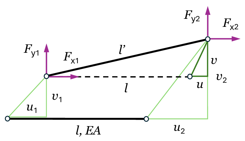
'We will formulate a 2D truss element with 3rd order geometric nonlinearity. The equilibrium equations will be derived in local CS, for the deformed state of the structure, assuming large displacements, as follows:
'<img style="height:115pt; width:198pt;" src="./Images/nonlin-truss-element.png" alt="nonlin-truss-element.png">
#noc
'Relative displacements -'u = u_2 - u_1', 'v = v_2 - v_1', 'z = [u; v]
#equ
'Length and elongation of the element in deformed state
l′(e; z) = sqrt((l(e) + z.1)^2 + z.2^2)','Δl(e; z) = l′(e; z) - l(e)', 'ε(e; z) = Δl(e; z)/l(e) + ε_P
'Directions of the displaced axis of the element in the deformed state
c_d(e; z) = (l(e) + z.1)/l′(e; z)', 's_d(e; z) = z.2/l′(e; z)
'Axial force in element -'N(e; z) = σ(ε(e; z))*A
'Horizontal reactive force at the right end -'F_x(e; z) = N(e; z)*c_d(e; z)
'Vertical reactive force at the right end -'F_y(e; z) = N(e; z)*s_d(e; z)
'Partial derivatives of element end reactive forces
F′_x1(e; z) = (1/l(e) - z.2^2/l′(e; z)^3)', ' _
F′_x2(e; z) = (z.2*(l(e) + z.1)/l′(e; z)^3)
F′_y1(e; z) = F′_x2(e; z)', ' _
F′_y2(e; z) = (1/l(e) - (l(e) + z.1)^2/l′(e; z)^3)
'We are not going to linearize the above equations by Taylor series. We will use them further directly in their implicit form.
'<h4>Solution by Newton-Raphson’s method</h4>
'We will express the parameters of the system as a function of the vector of t he unknown displacements:
Z = vector(2*n_J)*mm
'Initial deflection at the intermediate joint -'Z.(n_J + 1) = 100mm
'Extracting displacements for joint <var>j</var> -'z_J(j) = [Z.(2*j - 1); Z.(2*j)]
'Relative displacements for element <var>e</var> -' _
z_e(e) = t(e)*(z_J(J_2(e)) - z_J(J_1(e)))
'Element reactive forces partial vector -' _
F_e(e) = t(e)*[F_x(e; z_e(e)); F_y(e; z_e(e))]
'Partial element Jacobi matrix
J_e(e) = t(e)*[ _
F′_x1(e; z_e(e)); F′_x2(e; z_e(e))| _
F′_y1(e; z_e(e)); F′_y2(e; z_e(e))]
'Target precision -'ε_max = 10^-5
#hide
#for n = 1 : 100
    z_J(j) = [Z.(2*j - 1); Z.(2*j)]
    'Global load vector
    F = vector(2*n_J)*kN
    s = -1
    'Add internal forces
    #for e = 1 : n_E
        #for k = 1 : 2
            j = E_J.(e; k)
            j_2 = 2*j
            F.(j_2 - 1) = F.(j_2 - 1) + take(1; F_e(e))*s
            F.(j_2) = F.(j_2) + take(2; F_e(e))*s
            s = -s
        #loop
    #loop
    'Add support rections
    #for i = 1 : n_c
        j = c_J.(i; 1)
        j_2 = 2*j
        F.(j_2 - 1) = F.(j_2 - 1) + c_J.(i; 2)*Z.(j_2 - 1)
        F.(j_2) = F.(j_2) + c_J.(i; 3)*Z.(j_2)
    #loop
    'Add external loads
    #for i = 1 : n_F
        j = F_J.(i; 1)
        j_2 = 2*j
        F.(j_2 - 1) = F.(j_2 - 1) + F_J.(i; 2)
        F.(j_2) = F.(j_2) + F_J.(i; 3)
    #loop
    'Global Jacobi matrix
    J = symmetric(2*n_J)*kN/m
    'Add element Jacobi matrices
    #for e = 1 : n_E
        ε = ε(e; z_e(e))
        EA = if(ε < ε_y; EA_0; max(EA_0/10; EA_1))
        #for i = 1 : 2
            #for j = 1 : 2
                k = if(i ≡ j; EA; -EA)
                i_1 = 2*E_J.(e; i) - 1
                j_1 = 2*E_J.(e; j) - 1
                add(k*J_e(e); J; i_1; j_1)
            #loop
        #loop
    #loop
    'Add support springs
    #for i = 1 : n_c
        j = c_J.(i; 1)
        C_x = c_J.(i; 2)
        C_y = c_J.(i; 3)
        j_1 = 2*j - 1
        j_2 = 2*j
        J.(j_1; j_1) = J.(j_1; j_1) + C_x
        J.(j_2; j_2) = J.(j_2; j_2) + C_y
    #loop
    Z_0 = Z
    δZ = clsolve(J; F)|mm
    Z = Z_0 - δZ
    ε = norm_e(δZ)/norm_e(Z)
    #if ε < ε_max
        #break
    #end if
#loop
#show
'Iteratively calculate the following equations of the Newton-Raphson’s method:
#noc
Z_0 = Z','δZ = clsolve(J(Z); F(Z))|mm','Z = Z_0 - δZ','ε = norm_e(δZ)/norm_e(Z) < ε_max
#equ
'Convergence reached at iteration -'n'. Relative error -'ε
'<h4>Results</h4>
'<p><strong>Joint displacements</strong> -'Z(j) = round(z_J(j)/δz)*δz'</p>
#novar
#for j = 1 : n_J
    #if norm_1(Z(j)) > δz*mm
        #val
        '<p>Joint <b>J'j'</b> - <var>Z</var><sub>'j
        #equ
        '</sub> ='Z(j)'</p>
    #end if
#loop
#varsub
'<p><strong>Reactions in supports</strong></p>
r(i) = row(c_J; i)','j(i) = take(1; r(i))', ' _
R(i) = -z_J(j(i))*last(r(i); 2)
#novar
#for i = 1 : n_c
    #val
    '<p>Joint <b>J'j(i)'</b> - <var>R</var><sub>'i
    #equ
    '</sub> ='R(i)'</p>
#loop
#varsub
'Element yield capacity  -'N_y = f_y*A
'Element ultimate capacity -'N_u = f_u*A
'<p><strong>Element axial forces</strong> -'N_e(e) = N(e; z_e(e))'</p>
#novar
#for e = 1 : n_E
    #val
    '<p>Element <b>Е'e'</b> - <var>N</var><sub>'e'
    #equ
    '</sub> ='N_e(e)'</p>
#loop
#varsub
#val
#hide
k = W/w
δ = 0.5m*k
#show
svg$
'<polygon points="'0','0' '0','-3*δ' '-0.2*δ','-2.4*δ' '0.2*δ','-2.4*δ' '0','-3*δ'" load_style$/>
'<polygon points="'W','0' 'W','-3*δ' 'W - 0.2*δ','-2.4*δ' 'W + 0.2*δ','-2.4*δ' 'W','-3*δ'" load_style$/>
'<polygon points="'r','0' '-3*δ','0' '-2.4*δ','-0.2*δ' '-2.4*δ','0.2*δ' '-3*δ','0'" load_style$/>
'<polygon points="'W + r','0' 'W + 3*δ','0' 'W + 2.4*δ','-0.2*δ' 'W + 2.4*δ','0.2*δ' 'W + 3*δ','0'" load_style$/>
texth$(-2*δ;-0.5*δ;Rx='take(1; R(1))'kN)
texth$(W+2*δ;-0.5*δ;Rx='take(1; R(2))'kN)
texth$(2*δ;-3.2*δ;Ry='take(2; R(1))'kN)
texth$(W-2*δ;-3.2*δ;Ry='take(2; R(2))'kN)
frame$
'</svg>
#equ

Rendered Output:

Input data

⃗x_J = [0 m 3 m 9 m] , ⃗y_J = [0 m 0 m 0 m] , n_J = len ( ⃗x_J )  = 3

Elements - [J1; J2]

transp ( E_J )  = 12 23 , n_E = n_rows ( E_J )  = 2 , J₁ ( e )  = E_J.e,1 , J₂ ( e )  = E_J.e,2

Element endpoint coordinates

x₁ ( e )  = ⃗x_{J.J1  ( e )} , y₁ ( e )  = ⃗y_{J.J1  ( e )} , x₂ ( e )  = ⃗x_{J.J2  ( e )} , y₂ ( e )  = ⃗y_{J.J2  ( e )}

Element lengths - l ( e )  =    √  ( x₂  ( e )  − x₁  ( e )  ) ² +  ( y₂  ( e )  − y₁  ( e )  ) ²

Element directions - c ( e )  = x₂  ( e )  − x₁  ( e ) l  ( e )  , s ( e )  = y₂  ( e )  − y₁  ( e ) l  ( e ) 

Transformation matrix

t ( e )  = [c  ( e ) ; s  ( e )  | -s  ( e ) ; c  ( e ) ]

T ( e )  = add ( t  ( e ) ; add ( t  ( e ) ; matrix ( 4; 4 ) ; 1; 1 ) ; 3; 3 ) 

Supports - [Joint; cx; cy]

c_J = 110²⁰ kN ∕ m10²⁰ kN ∕ m 310²⁰ kN ∕ m10²⁰ kN ∕ m

n_c = n_rows ( c_J )  = 2

Material - steel

We assume bi-linear material model

Initial modulus of elasticity - E₀ = 206 GPa

Yield stress - f_y = 500 MPa

Ultimate tensile stress - f_u = 600 MPa

Yield strain - ε_y = f_yE₀ = 500 MPa206 GPa = 2.43 ‰

Ultimate strain - ε_u = 20 ‰

Modulus of elasticity after yield - E₁ = f_u − f_yε_u − ε_y = 600 MPa − 500 MPa20 ‰ − 2.43 ‰ = 5.69 GPa

Idealized stress-strain curve - σ ( ε )  = {if ε < ε_y: E₀ · ε
else: f_y + E₁ ·  ( ε − ε_y ) 

Cross section – circular with diameter Φ = 20 mm

Area - A = π · Φ²4 = 3.14 ·  ( 20 mm ) ²4 = 3.14 cm²

Stiffness

Initial - EA₀ = E₀ · A = 206 GPa · 3.14 cm² = 64716.8 kN , EA = EA₀ = 64716.8 kN

After yield - EA₁ = E₁ · A = 5.69 GPa · 3.14 cm² = 1787.76 kN

Load - [Joint, Fx, Fy]

F_J = 20 kN-70 kN , n_F = n_rows ( F_J )  = 1

Prestressing force - P = 20 kN

Initial stress - σ_P = PA = 20 kN3.14 cm² = 63.66 MPa

Initial strain - ε_P = σ_PE₀ = 63.66 MPa206 GPa = 0.000309

Finite element formulation

We will formulate a 2D truss element with 3rd order geometric nonlinearity. The equilibrium equations will be derived in local CS, for the deformed state of the structure, assuming large displacements, as follows:

Relative displacements - u = u₂ − u₁ , v = v₂ − v₁ , ⃗z = [u; v]

Length and elongation of the element in deformed state

l′ ( e; z )  =    √  ( l  ( e )  + z₁ ) ² + z₂² , Δl ( e; z )  = l′  ( e; z )  − l  ( e )  , ε ( e; z )  = Δl  ( e; z ) l  ( e )  + ε_P

Directions of the displaced axis of the element in the deformed state

c_d ( e; z )  = l  ( e )  + z₁l′  ( e; z )  , s_d ( e; z )  = z₂l′  ( e; z ) 

Axial force in element - N ( e; z )  = σ  ( ε  ( e; z )  )  · A

Horizontal reactive force at the right end - F_x ( e; z )  = N  ( e; z )  · c_d  ( e; z ) 

Vertical reactive force at the right end - F_y ( e; z )  = N  ( e; z )  · s_d  ( e; z ) 

Partial derivatives of element end reactive forces

F′_x1 ( e; z )  = 1l  ( e )  − z₂²l′  ( e; z ) ³ , F′_x2 ( e; z )  = z₂ ·  ( l  ( e )  + z₁ ) l′  ( e; z ) ³

F′_y1 ( e; z )  = F′_x2  ( e; z )  , F′_y2 ( e; z )  = 1l  ( e )  −  ( l  ( e )  + z₁ ) ²l′  ( e; z ) ³

We are not going to linearize the above equations by Taylor series. We will use them further directly in their implicit form.

Solution by Newton-Raphson’s method

We will express the parameters of the system as a function of the vector of t he unknown displacements:

⃗Z = vector ( 2 · n_J )  · mm = vector ( 2 · 3 )  · mm = [0 mm 0 mm 0 mm 0 mm 0 mm 0 mm]

Initial deflection at the intermediate joint - ⃗Z₄ = 100 mm

Extracting displacements for joint j - z_J ( j )  = [⃗Z_{2 · j − 1}; ⃗Z_2 · j]

Relative displacements for element e - z_e ( e )  = t  ( e )  ·  ( z_J  ( J₂  ( e )  )  − z_J  ( J₁  ( e )  )  ) 

Element reactive forces partial vector - F_e ( e )  = t  ( e )  · [F_x  ( e; z_e  ( e )  ) ; F_y  ( e; z_e  ( e )  ) ]

Partial element Jacobi matrix

J_e ( e )  = t  ( e )  · [F′_x1  ( e; z_e  ( e )  ) ; F′_x2  ( e; z_e  ( e )  )  | F′_y1  ( e; z_e  ( e )  ) ; F′_y2  ( e; z_e  ( e )  ) ]

Target precision - ε_max = 10^-5

Iteratively calculate the following equations of the Newton-Raphson’s method:

⃗Z₀ = ⃗Z , ⃗δZ = clsolve ( J  ( ⃗Z ) ; F  ( ⃗Z )  )  , ⃗Z = ⃗Z₀ − ⃗δZ , ε = norm_e ( ⃗δZ ) norm_e ( ⃗Z )  < ε_max

Convergence reached at iteration - n = 33 . Relative error - ε = 7.27×10^-6

Results

Joint displacements - Z ( j )  = round(z_J  ( j ) δz) · δz

Joint J2 - Z₂ = Z  ( 2 )  = [-44.7 mm 772.72 mm]

Reactions in supports

r ( i )  = row ( c_J; i )  , j ( i )  = take ( 1; r  ( i )  )  , R ( i )  = -z_J  ( j  ( i )  )  · last ( r  ( i ) ; 2 ) 

Joint J1 - R₁ = R  ( 1 )  = [-179.81 kN -47.01 kN]

Joint J3 - R₂ = R  ( 2 )  = [179.81 kN -22.99 kN]

Element yield capacity - N_y = f_y · A = 500 MPa · 3.14 cm² = 157.08 kN

Element ultimate capacity - N_u = f_u · A = 600 MPa · 3.14 cm² = 188.5 kN

Element axial forces - N_e ( e )  = N  ( e; z_e  ( e )  ) 

Element Е1 - N₁ = N_e  ( 1 )  = 185.86 kN

Element Е2 - N₂ = N_e  ( 2 )  = 181.27 kN

Nonlinear Analysis of a Von-Mises Truss 🎬

Shallow Von-Mises truss with circular pipe section, animated load-displacement curve passing through a limit point, solved by fixed-point iteration, Newton-Raphson, the secant method and the built-in Root solver.

Code:

'(solved by four different numerical methods)
'<h4>Input data</h4>
'Half span -'a = 2m', ''Height -'h = -0.5m
'Cross section - circular pipe with diameter'Φ = 100mm'and thickness't = 4mm
'Material - steel. Modulus of elasticity -'E = 210GPa
'Vertical force -'F_y = 2000kN
#include svg_drawing.cpd
#hide
v = 0mm
L = a/2cm
H = h/cm
H_lin = H
H_nl = H
k = L/10
W = 2*(L + 6*k)
Y = H
F_y,max = 2500kN
v_max = abs(2.26*h)
#def svg$ = '<svg viewbox="'-6*k' 'Y' 'W' 'abs(H)'" xmlns="http://www.w3.org/2000/svg" version="1.1" style="font-family: Georgia Pro; font-size:7px; width:'420'pt; height:'400*abs(H)/L'pt">
#def thin_style$ = style="stroke:darkcyan; stroke-width:1; fill:none;"
#def dash_style$ = style="stroke:#ddd; stroke-width:1; stroke-dasharray: 7 3; fill:none;"
#def ghost_style$ = style="stroke:#ddd; stroke-width:1; fill:white;"
#def lin_style$ = style="stroke:#ccc; stroke-width:2; fill:none;"
#def pin_style$ = style="stroke:red; stroke-width:1; fill:white;"
#def thick_style$ = style="stroke:darkcyan; stroke-width:3; fill:none;"
#def load_style$ = style="stroke:deepskyblue; stroke-width:1; fill:deepskyblue;"
#show
#def frame$
    line$(0; 0; L; H; dash_style$)
    line$(L; H; 2*L; 0; dash_style$)
    line$(0; 0; L; H_lin; lin_style$)
    line$(L; H_lin; 2*L; 0; lin_style$)
    circle$(L; H_lin; 2.5; ghost_style$)
    line$(0; 0; L; H_nl; main_style$)
    line$(L; H_nl; 2*L; 0; main_style$)
    #hide
    x1 = 0
    y1 = k/10
    #show
    #for i = 1 : 2
        #hide
        δ = 0.8*k
        x2 = x1 - δ
        y2 = y1 - abs(δ)
        x3 = x1 + δ
        y3 = y1 + abs(δ)
        #show
        line$(x2; y3; x3; y3; thick_style$)
        line$(x2; y3; x1; y1; thin_style$)
        line$(x3; y3; x1; y1; thin_style$)
        #hide
        x1 = x1 + 2*L
        #show
    #loop
    '<polygon points="'L','H_nl - 4*δ' 'L','H_nl - 0.32*δ' 'L - 0.32*δ','H_nl - 1.4*δ' 'L + 0.32*δ','H_nl - 1.4*δ' 'L','H_nl - 0.32*δ'" load_style$ />
    texth$(L+20;H_nl-3.2*δ;Fy='F_y'kN)
    dimh$(0; L; (1-2*sign(H_nl))*k; 'a'm)
    dimh$(L; 2*L; (1-2*sign(H_nl))*k; 'a'm)
    #if H_nl < 0
        dimv$(L - k; H_nl; 0; 'h + v'm)
    #else
        dimv$(L - k; 0; H_nl; 'h + v'm)
    #end if
    circle$(0; 0; 2.5; pin_style$)
    circle$(L; H_nl; 2.5; pin_style$)
    circle$(2*L; 0; 2.5; pin_style$)
#end def
#val
svg$
frame$
'</svg>
#equ
'<h4>Linear Solution</h4>
'Strut length -'l = srss(a; h)
'Area -'A = π*(Φ^2 - (Φ - 2*t)^2)/4|cm^2
'Axial stiffness -'EA = E*A
'Axial forces in bars -'N(F) = F*l/(2*h)', 'N(F_y)
'Vertical displacement -'v_l(F) = -sqrt((l + (N(F)*l)/EA)^2 - a^2) - h|mm
v_l(F_y)
'<h4>Nonlinear Solution</h4>
'The vertical displacement is the only unknown - <var>v</var> = ?
'We will use 3-rd order geometric nonlinearity theory for the solution. The equilibrium equations are then derived for the deformed state of the structure, as follows:
'Length and elongation in deformed state
l′(v) = sqrt(a^2 + (h + v)^2)','Δl(v) = l′(v) - l
'Horizontal reaction -'F_x(v) = EA*(Δl(v)/l)*(a/l′(v))
'Vertical reaction -'F_y(v) = EA*(Δl(v)/l)*((h + v)/l′(v))
'Vertical reaction derivative -'F′_yv(v) = EA*(1/l - a^2/l′(v)^3)
'<h4>1. Fixed point iteration method</h4>
'Relative strain -'ε = F_y/(2*EA)
'Relative precision -'δ_max = 10^-5
'Initial value -'v_0 = 1mm
'We express the unknown vertical displacement at the middle joint as a function of the vertical force:
v = sqrt(1/(1/l - ε/(h + v_0))^2 - a^2) - h|mm
#hide
n = 0
#repeat 100
    n = n + 1
    v_0 = v
    v = sqrt(1/(1/l - ε/(h + v_0))^2 - a^2) - h|mm
    δ = abs(v - v_0)
    #if δ < δ_max*abs(v)
        #break
    #end if
#loop
#show
'After calculating the above expression iteratively'n'times, we get:
v
'Relative error -'δ = abs(v - v_0)/abs(v)
'<h4>2. Newton-Raphson′s method</h4>
'Initial value -'v_0 = 0mm
'We repeatedly calculate the following expression:
v = v_0 - (2*F_y(v_0) - F_y)/F′_yv(v_0)
#hide
n = 0
#repeat 100
    n = n + 1
    v_0 = v
    v = v_0 - (2*F_y(v_0) - F_y)/(2*F′_yv(v_0))
    δ = abs(v - v_0)
    #if δ < δ_max*abs(v)
        #break
    #end if
#loop
#show
'After'n'iterations we get:'v
'Relative error -'δ = abs(v - v_0)/abs(v)
'<h4>3. Secant method</h4>
'Slope reduction factor -'α = 1
'Initial value -'v_0 = 0mm
'Force value -'F_y0 = 2*F_y(v_0)
'We calculate the first approximation using Newton-Raphson′s method
v_1 = v_0 - α*((F_y0 - F_y)/(2*F′_yv(v_0)))
'Force value -'F_y1 = 2*F_y(v_1)
'The next approximation is evaluated by the formula:
v_2 = v_1 - α*(F_y1 - F_y)*((v_1 - v_0)/(F_y1 - F_y0))
'We continue the calculations iteratively until we reach convergence.
#hide
n = 0
#repeat 100
    n = n + 1
    v_0 = v_1
    v_1 = v_2
    F_y0 = 2*F_y(v_0)
    F_y1 = 2*F_y(v_1)
    v_2 = v_1 - α*(F_y1 - F_y)*((v_1 - v_0)/(F_y1 - F_y0))
    δ = abs(v_2 - v_1)
    #if δ < δ_max*abs(v_2)
        #break
    #end if
#loop
#show
'After'n'iterations we get:'v_2
'Relative error -'δ = abs(v_2 - v_1)/abs(v_2)
'<h4>4. Solution with Calcpad <small>(modified Anderson-Bjork′s method)</small></h4>
v = $Root{2*F_y(v) = F_y @ v = 0mm : 200m}
'System behavior graph (force-displacement)
'<!--'PlotWidth = 400','PlotHeight = 180','ReturnAngleUnits = 1'-->
#def plot$
    #hide
    v_2 = v
    F′ = 2*F′_yv(v)
    dv = min(2000kN/F′; v_max/6)
    v_1(v) = min(max(0mm; v_2 + (1 - 2*v/v_max)*dv); v_max)
    F_1(v) = F_y + F′*(v_1(v) - v_2)
    #show
    $Plot{F_y & 2*F_y(v) & v_1(v)|F_1(v) & v_l(F_y)|F_y & v_2|F_y @ v = 0mm : v_max}
#end def
plot$
'<h4>Results</h4>
'Axial forces in bars -'N = Δl(v)/l*EA
'Rotation angle -'α = atan2(l; v)
'Reactions in supports
'Horizontal -'R_x = F_x(v)'='N*cos(α)
'Vertical -'R_y = F_y(v)'='N*sin(α)
#hide
L = a/2cm
k = L/10
δ = 0.7*k
#show
#val
#def results$
    #hide
    N = round(Δl(v)/l*EA)
    α = atan2(l; v)
    R_x = F_x(v)'='N*cos(α)
    R_y = F_y(v)'='N*sin(α)
    H_lin = (h + v_l(F_y))/cm
    H_nl = (h + v)/cm
    Y = H + 2*k
    #show
    svg$
    '<polygon points="'0','0' '0','-4*δ' '-0.32*δ','-2.8*δ' '0.32*δ','-2.8*δ' '0','-4*δ'" load_style$/>
    '<polygon points="'2*L','0' '2*L','-4*δ' '2*L - 0.32*δ','-2.8*δ' '2*L + 0.32*δ','-2.8*δ' '2*L','-4*δ'" load_style$/>
    '<polygon points="'-0.32*δ','0' '-4*δ','0' '-2.8*δ','-0.32*δ' '-2.8*δ','0.32*δ' '-4*δ','0'" load_style$/>
    '<polygon points="'2*L + 0.32*δ','0' '2*L + 4*δ','0' '2*L + 2.8*δ','-0.32*δ' '2*L + 2.8*δ','0.32*δ' '2*L + 4*δ','0'" load_style$/>
    texth$(-4*δ;-δ;Rx='round(R_x)'kN)
    texth$(2*L+4*δ;-δ;Rx='round(R_x)'kN)
    texth$(3.2*δ;-3.2*δ;Ry='round(R_y)'kN)
    texth$(2*L-3.2*δ;-3.2*δ;Ry='round(R_y)'kN)
    texth$(L/2;0;N='N'kN)
    texth$(3*L/2;0;N='N'kN)
    frame$
    '</svg>
#end def
results$
#hide
n = 51
#show
'<style>.fr{display:none;}</style>
#for j = 1 : n
    #hide
    F_y = F_y,max*(j - 1)/(n - 1)
    v = $Root{2*F_y(v) = F_y @ v = 0mm : 200m}
    #show
    '<div class="fr" id="fr-'j'">
    plot$
    results$
    '</div>
#loop
'<script>(function(){$("#fr-1").show();var i=1;var fr=$("#fr-1");setInterval(function(){fr.hide();if(++i>'n')i=1;fr=$("#fr-"+i);fr.show();}, 100);})();</script>
#equ

Rendered Output:

(solved by four different numerical methods)

Input data

Half span - a = 2 m , 'Height - h = -0.5 m

Cross section - circular pipe with diameter Φ = 100 mm and thickness t = 4 mm

Material - steel. Modulus of elasticity - E = 210 GPa

Vertical force - F_y = 2000 kN

Linear Solution

Strut length - l = srss ( a; h )  = srss ( 2 m; -0.5 m )  = 2.06 m

Area - A = π ·  ( Φ² −  ( Φ − 2 · t ) ² ) 4 = 3.14 ·  (  ( 100 mm ) ² −  ( 100 mm − 2 · 4 mm ) ² ) 4 = 12.06 cm²

Axial stiffness - EA = E · A = 210 GPa · 12.06 cm² = 253338 kN

Axial forces in bars - N ( F )  = F · l2 · h , N  ( F_y )  = N  ( 2000 kN )  = -4123.11 kN

Vertical displacement - v_l ( F )  = -  (l + N  ( F )  · lEA)² − a² − h

v_l  ( F_y )  = v_l  ( 2000 kN )  = 164.16 mm

Nonlinear Solution

The vertical displacement is the only unknown - v = ?

We will use 3-rd order geometric nonlinearity theory for the solution. The equilibrium equations are then derived for the deformed state of the structure, as follows:

Length and elongation in deformed state

l′ ( v )  =    √ a² +  ( h + v ) ² , Δl ( v )  = l′  ( v )  − l

Horizontal reaction - F_x ( v )  = EA · Δl  ( v ) l · al′  ( v ) 

Vertical reaction - F_y ( v )  = EA · Δl  ( v ) l · h + vl′  ( v ) 

Vertical reaction derivative - F′_yv ( v )  = EA · (1l − a²l′  ( v ) ³)

1. Fixed point iteration method

Relative strain - ε = F_y2 · EA = 2000 kN2 · 253338 kN = 0.00395

Relative precision - δ_max = 10^-5

Initial value - v₀ = 1 mm

We express the unknown vertical displacement at the middle joint as a function of the vertical force:

v =   1(1l − εh + v₀)² − a² − h =   1(12.06 m − 0.00395-0.5 m + 1 mm)² −  ( 2 m ) ² −  ( -0.5 m )  = 838.68 mm

After calculating the above expression iteratively n = 7 times, we get:

v = 1105.47 mm

Relative error - δ = | v − v₀ || v | = | 1105.47 mm − 1105.46 mm || 1105.47 mm | = 7.98×10^-6

2. Newton-Raphson′s method

Initial value - v₀ = 0 mm

We repeatedly calculate the following expression:

v = v₀ − 2 · F_y  ( v₀ )  − F_yF′_yv  ( v₀ )  = 0 mm − 2 · F_y  ( 0 mm )  − 2000 kNF′_yv  ( 0 mm )  = 276.68 mm

After n = 37 iterations we get: v = 1105.46 mm

Relative error - δ = | v − v₀ || v | = | 1105.46 mm − 1105.46 mm || 1105.46 mm | = 9.67×10^-10

3. Secant method

Slope reduction factor - α = 1

Initial value - v₀ = 0 mm

Force value - F_y0 = 2 · F_y  ( v₀ )  = 2 · F_y  ( 0 mm )  = 0 kN

We calculate the first approximation using Newton-Raphson′s method

v₁ = v₀ − α · F_y0 − F_y2 · F′_yv  ( v₀ )  = 0 mm − 1 · 0 kN − 2000 kN2 · F′_yv  ( 0 mm )  = 138.34 mm

Force value - F_y1 = 2 · F_y  ( v₁ )  = 2 · F_y  ( 138.34 mm )  = 1273.37 kN

The next approximation is evaluated by the formula:

v₂ = v₁ − α ·  ( F_y1 − F_y )  · v₁ − v₀F_y1 − F_y0 = 138.34 mm − 1 ·  ( 1273.37 kN − 2000 kN )  · 138.34 mm − 0 mm1273.37 kN − 0 kN = 217.28 mm

We continue the calculations iteratively until we reach convergence.

After n = 37 iterations we get: v₂ = 1105.46 mm

Relative error - δ = | v₂ − v₁ || v₂ | = | 1105.46 mm − 1105.46 mm || 1105.46 mm | = 2.28×10^-7

4. Solution with Calcpad (modified Anderson-Bjork′s method)

v = $Root{2 · F_y  ( v )  = F_y; v ∈ [0 mm; 200 m]} = 1105.46 mm

System behavior graph (force-displacement)

Results

Axial forces in bars - N = Δl  ( v ) l · EA = Δl  ( 1105.46 mm ) 2.06 m · 253338 kN = 3451.3 kN

Rotation angle - α = atan2 ( l; v )  = atan2 ( 2.06 m; 1105.46 mm )  = 28.2°

Reactions in supports

Horizontal - R_x = F_x  ( v )  = F_x  ( 1105.46 mm )  = 3303.25 kN = N · cos ( α )  = 3451.3 kN · cos ( 28.2° )  = 3041.6 kN

Vertical - R_y = F_y  ( v )  = F_y  ( 1105.46 mm )  = 1000 kN = N · sin ( α )  = 3451.3 kN · sin ( 28.2° )  = 1630.99 kN

Third Order Geometric Nonlinearity Analysis of a Double-Strut Biot System

Symmetric two-bar Biot truss in third-order geometric nonlinearity: the deformed length \(l'(v) = \sqrt{l^2 + v^2}\) enters the equilibrium directly and the vertical displacement is found by four different numerical methods.

Code:

'(solved by four different numerical methods)
'<h4>Input data</h4>
'Strut length -'l = 2m
'Material - steel. Modulus of elasticity -'E = 210GPa
'Cross section - circular with diameter'Φ = 20mm
'Area -'A = π*Φ^2/4|cm^2
'Axial stiffness -'EA = E*A
'Vertical force -'F_y = 20kN
#include svg_drawing.cpd
#hide
L = l/2cm
H = 0
k = L/10
#def svg$ = '<svg viewbox="'-5*k' '-5*k' '2*(L+5*k)' '10*k + H'" xmlns="http://www.w3.org/2000/svg" version="1.1" style="font-family: Georgia Pro; font-size:8px; width:'450'pt; height:'150'pt">
#def thin_style$ = style="stroke:darkcyan; stroke-width:1; fill:none"
#def pin_style$ = style="stroke:red; stroke-width:1; fill:white"
#def thick_style$ = style="stroke:darkcyan; stroke-width:3; fill:none"
#def load_style$ = style="stroke:deepskyblue; stroke-width:1; fill:deepskyblue;"
#show
#def frame$
    line$(0; 0; L; H; main_style$)
    line$(L; H; 2*L; 0; main_style$)
    #hide
    x1 = 0
    y1 = k/10
    #show
    #for i = 1 : 2
        #hide
        δ = 0.8*k
        x2 = x1 - δ
        y2 = y1 - abs(δ)
        x3 = x1 + δ
        y3 = y1 + abs(δ)
        #show
        line$(x2; y3; x3; y3; thick_style$)
        line$(x2; y3; x1; y1; thin_style$)
        line$(x3; y3; x1; y1; thin_style$)
        #hide
        x1 = x1 + 2*L
        #show
    #loop
    '<polygon points="'L','H - 4*δ' 'L','H - 0.32*δ' 'L - 0.32*δ','H - 1.4*δ' 'L + 0.32*δ','H - 1.4*δ' 'L','H - 0.32*δ'" load_style$ />
    texth$(L+20;H-3.2*δ;Fy='F_y'kN)
    dimh$(0; L; H+2*k; 'l'm)
    dimh$(L; 2*L; H+2*k; 'l'm)
    circle$(0; 0; 2.5; pin_style$)
    circle$(L; H; 2.5; pin_style$)
    circle$(2*L; 0; 2.5; pin_style$)
#end def
#val
svg$
frame$
'</svg>
#equ
'<h4>Solution</h4>
'Because of the symmetry, the horizontal displacement in the middle is'u = 0m'.
'The vertical displacement is the only unknown - <var>v</var> = ?
'Since the system is linearly unstable, we use 3-rd order geometric nonlinearity theory for the solution. The equilibrium equations are then derived for the deformed state of the structure, as follows:
'Length and elongation in deformed state
l′(v) = sqrt((l + u)^2 + v^2)','Δl(v) = l′(v) - l
'Horizontal reaction -'F_x(v) = EA*(Δl(v)/l)*((l + u)/l′(v))
'Vertical reaction -'F_y(v) = EA*(Δl(v)/l)*(v/l′(v))
'Vertical reaction derivative -'F′_yv(v) = EA*(1/l - (l + u)^2/l′(v)^3)
'<h4>1. Fixed point iteration method</h4>
'Relative strain -'ε = F_y/(2*EA)
'Relative precision -'δ_max = 10^-4
'Initial value -'v_0 = 200mm
'We express the unknown vertical displacement at the middle joint as a function of the vertical force:
v = sqrt(1/(1/l - ε/v_0)^2 - (l + u)^2)|mm
#hide
n = 0
#repeat 100
    n = n + 1
    v_0 = v
    v = sqrt(1/(1/l - ε/v_0)^2 - (l + u)^2)|mm
    δ = abs(v - v_0)
    #if δ < δ_max*abs(v)
        #break
    #end if
#loop
#show
'After calculating the above expression iteratively'n'times, we get:
v
'Relative error -'δ = abs(v - v_0)/abs(v)
'<h4>2. Newton-Raphson′s method</h4>
'Initial value -'v_0 = 200mm
'We repeatedly calculate the following expression:
v = v_0 - (2*F_y(v_0) - F_y)/F′_yv(v_0)
#hide
n = 0
#repeat 100
    n = n + 1
    v_0 = v
    v = v_0 - (2*F_y(v_0) - F_y)/(2*F′_yv(v_0))
    δ = abs(v - v_0)
    #if δ < δ_max*abs(v)
        #break
    #end if
#loop
#show
'After'n'iterations we get:'v
'Relative error -'δ = abs(v - v_0)/abs(v)
'<h4>3. Secant method</h4>
'Slope reduction factor -'α = 1
'Initial value -'v_0 = 200mm
'Force value -'F_y0 = 2*F_y(v_0)
'We calculate the first approximation using Newton-Raphson′s method
v_1 = v_0 - α*((F_y0 - F_y)/(2*F′_yv(v_0)))
'Force value -'F_y1 = 2*F_y(v_1)
'The next approximation is evaluated by the formula:
v_2 = v_1 - α*(F_y1 - F_y)*((v_1 - v_0)/(F_y1 - F_y0))
'We continue the calculations iteratively until we reach convergence.
#hide
n = 0
#repeat 100
    n = n + 1
    v_0 = v_1
    v_1 = v_2
    F_y0 = 2*F_y(v_0)
    F_y1 = 2*F_y(v_1)
    v_2 = v_1 - α*(F_y1 - F_y)*((v_1 - v_0)/(F_y1 - F_y0))
    δ = abs(v_2 - v_1)
    #if δ < δ_max*abs(v_2)
        #break
    #end if
#loop
#show
'After'n'iterations we get:'v_2
'Relative error -'δ = abs(v_2 - v_1)/abs(v_2)
'<h4>4. Solution with Calcpad <small>(modified Anderson-Bjork′s method)</small></h4>
v = $Root{2*F_y(v) = F_y @ v = 0mm : 200m}
'System behavior graph (force-displacement)
'<!--'v_2 = v','PlotWidth = 250','PlotHeight = 150'-->
$Plot{F_y & 2*F_y(v) & v_2|F_y @ v = 0mm : 200mm}
'<h4>Results</h4>
'Axial forces in bars -'N = Δl(v)/l*EA
'Rotation angle -'α = atan2(l; v)'°
'Reactions in supports
'Horizontal -'R_x = F_x(v)'='N*cos(α)
'Vertical -'R_y = F_y(v)'='N*sin(α)
#hide
H = v/cm
δ = 0.8*k
#show
#val
svg$
'<polygon points="'0','0' '0','-4*δ' '-0.32*δ','-2.8*δ' '0.32*δ','-2.8*δ' '0','-4*δ'" load_style$/>
'<polygon points="'2*L','0' '2*L','-4*δ' '2*L - 0.32*δ','-2.8*δ' '2*L + 0.32*δ','-2.8*δ' '2*L','-4*δ'" load_style$/>
'<polygon points="'-0.32*δ','0' '-4*δ','0' '-2.8*δ','-0.32*δ' '-2.8*δ','0.32*δ' '-4*δ','0'" load_style$/>
'<polygon points="'2*L + 0.32*δ','0' '2*L + 4*δ','0' '2*L + 2.8*δ','-0.32*δ' '2*L + 2.8*δ','0.32*δ' '2*L + 4*δ','0'" load_style$/>
texth$(-4*δ;-δ;Rx='R_x'kN)
texth$(2*L+4*δ;-δ;Rx='R_x'kN)
texth$(3*δ;-3.2*δ;Ry='R_y'kN)
texth$(2*L-3*δ;-3.2*δ;Ry='R_y'kN)
texth$(L/2;0;N='N'kN)
texth$(3*L/2;0;N='N'kN)
frame$
'</svg>
#equ

Rendered Output:

Solution

Because of the symmetry, the horizontal displacement in the middle is u = 0 m .

The vertical displacement is the only unknown - v = ?

Since the system is linearly unstable, we use 3-rd order geometric nonlinearity theory for the solution. The equilibrium equations are then derived for the deformed state of the structure, as follows:

Length and elongation in deformed state

l′ ( v )  =    √  ( l + u ) ² + v² , Δl ( v )  = l′  ( v )  − l

Horizontal reaction - F_x ( v )  = EA · Δl  ( v ) l · l + ul′  ( v ) 

Vertical reaction - F_y ( v )  = EA · Δl  ( v ) l · vl′  ( v ) 

Vertical reaction derivative - F′_yv ( v )  = EA · (1l −  ( l + u ) ²l′  ( v ) ³)

1. Fixed point iteration method

Relative strain - ε = F_y2 · EA = 20 kN2 · 65973.4 kN = 0.000152

Relative precision - δ_max = 10^-4 = 0.0001

Initial value - v₀ = 200 mm

We express the unknown vertical displacement at the middle joint as a function of the vertical force:

v =   1(1l − εv₀)² −  ( l + u ) ² =   1(12 m − 0.000152200 mm)² −  ( 2 m + 0 m ) ² = 110.24 mm

After calculating the above expression iteratively n = 13 times, we get:

v = 134.51 mm

Relative error - δ = | v − v₀ || v | = | 134.51 mm − 134.5 mm || 134.51 mm | = 7.6×10^-5

2. Newton-Raphson′s method

Initial value - v₀ = 200 mm

We repeatedly calculate the following expression:

v = v₀ − 2 · F_y  ( v₀ )  − F_yF′_yv  ( v₀ )  = 200 mm − 2 · F_y  ( 200 mm )  − 20 kNF′_yv  ( 200 mm )  = 106.93 mm

After n = 4 iterations we get: v = 134.51 mm

Relative error - δ = | v − v₀ || v | = 9×10^-6

3. Secant method

Slope reduction factor - α = 1

Initial value - v₀ = 200 mm

Force value - F_y0 = 2 · F_y  ( v₀ )  = 2 · F_y  ( 200 mm )  = 65.48 kN

We calculate the first approximation using Newton-Raphson′s method

v₁ = v₀ − α · F_y0 − F_y2 · F′_yv  ( v₀ )  = 200 mm − 1 · 65.48 kN − 20 kN2 · F′_yv  ( 200 mm )  = 153.46 mm

Force value - F_y1 = 2 · F_y  ( v₁ )  = 2 · F_y  ( 153.46 mm )  = 29.67 kN

The next approximation is evaluated by the formula:

v₂ = v₁ − α ·  ( F_y1 − F_y )  · v₁ − v₀F_y1 − F_y0 = 153.46 mm − 1 ·  ( 29.67 kN − 20 kN )  · 153.46 mm − 200 mm29.67 kN − 65.48 kN = 140.89 mm

We continue the calculations iteratively until we reach convergence.

After n = 4 iterations we get: v₂ = 134.51 mm

Relative error - δ = | v₂ − v₁ || v₂ | = | 134.51 mm − 134.51 mm || 134.51 mm | = 1.57×10^-6

4. Solution with Calcpad (modified Anderson-Bjork′s method)

v = $Root{2 · F_y  ( v )  = F_y; v ∈ [0 mm; 200 m]} = 134.51 mm

System behavior graph (force-displacement)

Results

Axial forces in bars - N = Δl  ( v ) l · EA = Δl  ( 134.51 mm ) 2 m · 65973.4 kN = 149.03 kN

Rotation angle - α = atan2 ( l; v )  = atan2 ( 2 m; 134.51 mm )  = 3.85 °

Reactions in supports

Horizontal - R_x = F_x  ( v )  = F_x  ( 134.51 mm )  = 148.69 kN = N · cos ( α )  = 149.03 kN · cos ( 3.85 )  = 148.69 kN

Vertical - R_y = F_y  ( v )  = F_y  ( 134.51 mm )  = 10 kN = N · sin ( α )  = 149.03 kN · sin ( 3.85 )  = 10 kN

Spotted an error? Edit these examples.