Parametric Curves¶

CalcpadCE plots parametric curves directly from their $x(t)$, $y(t)$ definitions: pick a parameter range, hand the two functions to $Plot, and the worksheet renders the trace inline.

This group walks through six classic families. The common spirals page surveys Archimedean, logarithmic, hyperbolic and Fermat spirals on a single canvas, while the Cornu spiral (Euler spiral) page traces the clothoid used in highway and railway transitions. The cycloidal pair — epicycloid and hypocycloid — generates the curves swept by a point on a circle rolling around or inside another, with rational ratios producing closed figures. Lissajous curves overlay two perpendicular harmonic motions to recreate oscilloscope patterns, and rose curves draw the petalled trace $r = a\, \cos(k\theta)$ that fills the polar plane.

Each worksheet exposes the shape parameters at the top, so changing one number redraws the curve immediately.

Common Spirals¶

Side-by-side plots of the Archimedean, logarithmic, hyperbolic and Fermat spirals on the same canvas, parameterised in polar form $r(\theta)$.

Code:

#hide
#rad
r(θ) = 1
#show
'General parametric equation:
x(θ) = r(θ)*cos(θ)
y(θ) = r(θ)*sin(θ)
'The radius <i>r</i>(<i>θ</i>) if different for each type of curve:
'Archimedes spiral - 'r(θ) = θ
#hide
PlotWidth = 400
PlotHeight = 390
#post
$Plot{x(θ)|y(θ) @ θ = 0 : 8*π}
#show
'Fermat spiral - 'r(θ) = sqr(θ)
#hide
PlotHeight = 387
#post
$Plot{x(θ)|y(θ) & -x(θ)|-y(θ) @ θ = 0 : 8*π}
#show
'Logarithmic spiral -'r(θ) = e^(a*θ)
#hide
a = 0.3
φ = (1 + sqr(5))/2
PlotHeight = 259
#post
$Plot{x(θ)|y(θ) @ θ = 0 : 8*π}
#show
'Golden spiral -'r(θ) = φ^(2/π*θ)
#hide
PlotHeight = 255
#post
$Plot{x(θ)|y(θ) @ θ = 0 : 8*π}
#show
'Hyperbolic spiral -'r(θ) = 1/θ
#hide
PlotHeight = 177
#post
$Plot{x(θ)|y(θ) @ θ = π/8 : 8*π}
#show
'Lituus -'r(θ) = 1/sqr(θ)
#hide
PlotHeight = 188
#post
$Plot{x(θ)|y(θ) @ θ = π/16 : 16*π}
#pre

'Tip: Click "<b>Calculate</b>" to see the respective plot.

Cornu Spiral¶

Plots the Cornu (Euler) spiral from the Fresnel integrals $C(t)$ and $S(t)$, the clothoid used as a transition curve in highway and railway alignment.

Code:

'(also <strong>Clothoid</strong> or <strong>Euler Spiral</strong>)
#rad
'The equations is defined by the Fresnel integrals:
x(t) = $Integral{cos(s^2) @ s = 0 : t}
y(t) = $Integral{sin(s^2) @ s = 0 : t}
#hide
PlotWidth = 440
PlotHeight = 400
#post
$Plot{x(t)|y(t) @ t = 0 : 2*π}
#pre

'Tip: Click "<b>Calculate</b>" to see the respective plot.

Epicycloid¶

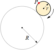
Trace of an epicycloid: the curve swept by a point on a small circle rolling on the outside of a fixed circle, with rational radius ratios producing closed figures.

Code:

'<div style="max-width:150mm">
'<img class="side" src="../../Images/math/epicycloid.png" alt="epicycloid.png">
'<p style="max-width:85mm">Epicycloid is a parametric curve that is obtained by rolling a smaller circle (<var>r</var>) around a larger one (<var>R</var>). It shows the trace of a point P, fixed on the circumference of the smaller circle.</p>
'General equation:
x(θ) = (k + 1)*cos(θ) - cos((k + 1)*θ)
y(θ) = (k + 1)*sin(θ) - sin((k + 1)*θ)
'Larger radius: 'R = ?
'Smaller radius: 'r = ?
'Ratio: 'k = R/r
#pre

'Tip: Click "<b>Calculate</b>" to see the respective plot.
#hide
#rad
PlotHeight = 400
PlotWidth = 400
#post
$Plot{x(θ)|y(θ) @ θ = 0 : 2*π*r}
#show
'</div>21   10

Hypocycloid¶

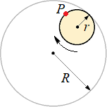
Trace of a hypocycloid: the curve swept by a point on a small circle rolling inside a fixed circle, including the astroid and deltoid as special cases.

Code:

'<div style="max-width:150mm">
'<img class="side" src="../../Images/math/hypocycloid.png" alt="hypocycloid.png">
'<p style="max-width:90mm">Hypocycloid is a parametric curve that is obtained by rolling a smaller circle (<var>r</var>) inside a larger one (<var>R</var>). It shows the trace of a point P, fixed on the circumference of the smaller circle.</p>
'General equation:
x(θ) = (k - 1)*cos(θ) + cos((k - 1)*θ)
y(θ) = (k - 1)*sin(θ) - sin((k - 1)*θ)
'Outer radius: 'R = ?
'Inner radius: 'r = ?
'Ratio: 'k = R/r
#pre

'Tip: Click "<b>Calculate</b>" to see the respective plot.
#hide
#rad
PlotHeight = 400
PlotWidth = 400
#post
$Plot{x(θ)|y(θ) @ θ = 0 : 2*π*r}
#show
'</div>22   3

Lissajous Curve¶

Two perpendicular harmonic motions $x = A\sin(a t + \delta)$, $y = B\sin(b t)$ overlaid to recreate classic Lissajous oscilloscope figures.

Code:

#hide
#rad
PlotHeight = 400
PlotWidth = 400
#show
'Equation:
x(θ) = sin(a*θ)
y(θ) = sin(b*θ)
'Coefficients:'a = ?','b = ?
#pre

'Tip: Click "<b>Calculate</b>" to see the respective plot.
#post
$Plot{x(θ)|y(θ) @ θ = 0 : 2*π}2   3

Rose Curve¶

Polar rose curve $r = a\, \cos(k\theta)$ with petal count controlled by integer or rational $k$.

Code:

'General equation:
r(θ) = cos(a/b*θ)
x(θ) = r(θ)*cos(θ)
y(θ) = r(θ)*sin(θ)
#pre
'<p>Coefficients <i>a</i>/<i>b</i> =
'<select data-target="ab">
'<option value="2;1">2</option>
'<option value="3;1">3</option>
'<option value="4;1">4</option>
'<option value="5;1">5</option>
'<option value="6;1">6</option>
'<option value="7;1">7</option>
'<option value="3;2">3/2</option>
'<option value="5;2">5/2</option>
'<option value="7;2">7/2</option>
'<option value="2;3">2/3</option>
'<option value="4;3">4/3</option>
'<option value="5;3">5/3</option>
'<option value="7;3">7/3</option>
'<option value="3;4">3/4</option>
'<option value="5;4">5/4</option>
'<option value="7;4">7/4</option>
'<option value="2;5">2/5</option>
'<option value="3;5">3/5</option>
'<option value="4;5">4/5</option>
'<option value="6;5">6/5</option>
'<option value="7;5">7/5</option>
'<option value="5;6">5/6</option>
'<option value="7;6">7/6</option>
'<option value="2;7">2/7</option>
'<option value="3;7">3/7</option>
'<option value="4;7">4/7</option>
'<option value="5;7">5/7</option>
'<option value="6;7">6/7</option>
'</select></p>
'<p style="display:none;" id="ab">'a = ? {4}','b = ? {1}'</span></p>

'Tip: Click "<b>Calculate</b>" to see the respective plot.
#hide
#rad
PlotHeight = 400
PlotWidth = 400
k = b*(1 + abs(a⦼2 - b⦼2))
#post
#val
'Coefficients <i>a</i>/<i>b</i> ='a'/'b
$Plot{x(θ)|y(θ) @ θ = 0 : k*π}

Spotted an error? Edit these examples.