Numerical¶

CalcpadCE treats numerical methods as first-class citizens: built-in operators such as $Slope, $Derivative, $Integral and $Find, paired with vector and matrix primitives, let you build classical algorithms from the ground up and watch every intermediate step.

This category collects recurring themes of applied analysis — root finding and eigenvalue extraction, quadrature and differentiation, regression and stochastic sampling — each captured in a self-contained, parametric worksheet. Iteration is treated as a visible artefact: Newton's method animates its convergence step-by-step, while Monte-Carlo experiments replace deterministic refinement with statistical accumulation. Comparison sheets pit competing formulas against analytical references, exposing the accuracy-versus-cost trade-off behind every algorithm.

Sample size, tolerances and iteration counts are exposed at the top of every sheet, so each worksheet doubles as a numerical playground for convergence, stability and round-off experiments.

Monte Carlo Pi¶

Estimates $\pi$ by sampling random points in the unit square and counting those falling inside the quarter circle. Includes a live SVG plot of the sample cloud coloured by inside-versus-outside membership, so accuracy and variance can be eyeballed at any sample size.

Code:

'Number of points -'n = 10000
'Point coordinates:
x = random(fill(vector_hp(n); 1))
y = random(fill(Vector_hp(n); 1))
'Point radii -'r = sqrt(x^2 + y^2)
'Result -'n_in = count(floor(r); 0; 1)', 'π_MC = 4*n_in/n
#val
#round 15
'<svg xmlns="http://www.w3.org/2000/svg" width="300" height="300" viewBox="-0.1 -0.1 1.2 1.2">
#for i = 1 : n
    '<circle cx="'x.i'" cy="'1 - y.i'" r="0.002" stroke="none"
    #if r.i < 1
        'fill = "red"/>
    #else
        'fill = "blue"/>
    #end if
#loop
'<rect x="0" y="0" width="1" height="1" fill="none" stroke="black" stroke-width="0.005"/>
'<path d="M 0 0 A 1 1 0 0 1 1 1" fill="none" stroke="black" stroke-width="0.005"/>
'</svg>

Rendered Output:

Number of points - n = 10000

Point coordinates:

⃗x = random ( fill ( vector_hp ( n ) ; 1 ) ) = random ( fill ( vector_hp ( 10000 ) ; 1 ) ) = [0.0543 0.183 0.254 0.164 0.207 0.471 0.815 0.575 0.612 0.762 0.814 0.256 0.597 0.152 0.0309 0.82 0.039 0.546 0.278 0.902 ... 0.146]

⃗y = random ( fill ( Vector_hp ( n ) ; 1 ) ) = random ( fill ( Vector_hp ( 10000 ) ; 1 ) ) = [0.806 0.45 0.33 0.0765 0.322 0.297 0.466 0.445 0.781 0.936 0.449 0.95 0.256 0.266 0.546 0.419 0.271 0.405 0.381 0.941 ... 0.896]

Point radii - ⃗r = √ ⃗x^⊙ 2 + ⃗y^⊙ 2 = [0.808 0.486 0.416 0.181 0.383 0.557 0.939 0.728 0.992 1.21 0.929 0.984 0.65 0.306 0.547 0.921 0.274 0.679 0.472 1.3 ... 0.908]

Result - n_in = count ( floor ( ⃗r ) ; 0; 1 ) = 7903 , π_MC = 4 · n_inn = 4 · 790310000 = 3.16

Newton's Method 🎬¶

Solves $x^x = 10$ with Newton iteration and renders an animated SVG that highlights each tangent step. The frame loop turns convergence into a visual sequence rather than a printed iteration table.

Code:

#md on
#noc
'**Problem:** Given the following equation:'x^x = 10'. Find'x'= ?              </p><p>
#equ
'**Solution:** Transform the equation in the form:'f(x) = x^x - 10'= 0</p>
'The first derivative is'f′(x) = x^x*(ln(x) + 1)
'Initial guess -'x_0 = 4', target precision -'δ = 10^-14
'#### Animation
'<style>#start{height:1.8em; padding-top:0;} .fr{display:none;} .Series3, .Series6{opacity:0;} .Series7{stroke-width:6pt;}</style>
#hide
#val
PlotWidth = 500','PlotHeight = 250','PlotSVG = 1','PlotAdaptive = 0
n = 100','x = x_0','a = 2','b = 4
#for i = 1 : n
    y_0 = f(x_0)
    #if i⦼2 ≡ 0
        x = x_0 - f(x_0)/f′(x_0)
        y = f(x)
        y(x) = y_0 + (x - x_0)*f′(x_0)
        #show
        '<div class="fr" id="fr-'i'">
        $Plot{f(ξ) & ξ|if(ξ ≥ x ∧ ξ ≤ x_0; y(ξ); 1/0) & 2|-50 & x|(ξ - a)*y/(b - a) & x|y & x_0|y_0 & x_0|y_0 @ ξ = a : b}
        '</div>
        #hide
        x_0 = x
    #else
        #if abs(y_0) < δ
            n = i - 4
            #break
        #end if
        #show
        '<div class="fr" id="fr-'i'">
        $Plot{f(ξ) & x_0|y_0 & 2|-50 & x_0|(ξ - a)*y_0/(b - a) & x_0|y_0 & x_0|y_0 & x_0|y_0 @ ξ = a : b}
        '</div>
        #hide
    #end if
#loop
#show
#equ
'After 'n' iterations we get:'x
'Check -'x^x', Error -'abs(x^x - 10)'<'δ
#val
'<script>(function(){$("#fr-1").show();var i=1;var fr=$("#fr-1");setInterval(function(){fr.hide();if(++i>'n')i=1;fr=$("#fr-"+i);fr.show();},1000);})();</script>

Rendered Output:

Problem: Given the following equation: x^x = 10 . Find x = ?

Solution: Transform the equation in the form: f ( x ) = x^x − 10 = 0

The first derivative is f′ ( x ) = x^x · ( ln ( x ) + 1 )

Initial guess - x₀ = 4 , target precision - δ = 10^-14

Animation

After n = 13 iterations we get: x = 2.51

Check - x^x = 2.51^2.51 = 10 , Error - | x^x − 10 | = | 2.51^2.51 − 10 | = 8.88×10^-15 < δ = 10^-14

Least Squares Fitting¶

Fits a 10-point dataset with linear, quadratic and quintic polynomial models built from the normal equations $X^T\, X\, a = X^T y$. All three curves are then plotted together so the residual pattern of each model is immediately visible.

Code:

'Point coordinates
x = [0; 1; 2; 3; 4; 5; 6; 7; 8; 9]
y = [400; 450; 440; 400; 380; 330; 250; 200; 150; 160]
'Number of points -'n = len(x)
e = fill(vector(n); 1)
'<h4>Linear fit</h4>
X = [e|x]
A = copy(X*transp(X); symmetric(n_rows(X)); 1; 1)
b = X*y
a_L = clsolve(A; b)
P_L(x) = dot(a_L; [1; x])
'<h4>Quadratic fit</h4>
X = [e|x|x^2]
A = copy(X*transp(X); symmetric(n_rows(X)); 1; 1)
b = X*y
a_Q = clsolve(A; b)
P_Q(x) = dot(a_Q; [1; x; x^2])
'<h4>Poly(5) fit</h4>
X = [e|x|x^2|x^3|x^4|x^5]
A = copy(X*transp(X); symmetric(n_rows(X)); 1; 1)
b = X*y
a_C = clsolve(A; b)
P_C(x) = dot(a_C; [1; x; x^2; x^3; x^4; x^5])
'<h4>Plot</h4>
#hide
PlotWidth = 250
PlotHeight = 150
#def P$ = x.1|y.1 & x.2|y.2 & x.3|y.3 & x.4|y.4 & x.5|y.5 & x.6|y.6 & x.7|y.7 & x.8|y.8 & x.9|y.9 & x.10|y.10
#show
$Plot{ξ|P_L(ξ) & P$ @ ξ = x.1 : x.n}
$Plot{ξ|P_Q(ξ) & P$ @ ξ = x.1 : x.n}
$Plot{ξ|P_C(ξ) & P$ @ ξ = x.1 : x.n}

Numerical Differentiation¶

Compares the $Slope operator (Richardson extrapolation) against $Derivative (complex-step method) on $e^x$ and $\sin(x^2)$ at large arguments. Exposes the round-off blow-up of finite differences and the machine-precision accuracy of the complex-step trick.

Code:

#md on
#rad
'Function -'f(x) = e^x', Point - 'a = 100
'Theoretical value -'f′(x) = e^x', 'y′_a = f′(a)
'**$Slope** function (Richardson extrapolation) -'y′_aS = $Slope{f(x) @ x = a}
'> Error -'δ = abs(y′_a - y′_aS)/y′_a|%'- <span class="err">Approx.</span>
'**$Derivative** function (Complex step method) -'y′_aD = $Derivative{f(x) @ x = a}
'> Error -'δ = abs(y′_a - y′_aD)/y′_a|%'- <span class="ok">Exact!!!</span>
'Function -'f(x) = sin(x^2)', Point -'a = 1000
'Theoretical value -'f′(x) = 2*x*cos(x^2)', 'y′_a = f′(a)
'**$Slope** function (Richardson extrapolation) -'y′_aS = $Slope{f(x) @ x = a}
'> Error -'δ = abs(y′_a - y′_aS)/y′_a|%'- <span class="err">Approx.</span>
'**$Derivative** function (Complex step method) -'y′_aD = $Derivative{f(x) @ x = a}
'> Error -'δ = abs(y′_a - y′_aD)/y′_a|%'- <span class="ok">Exact!!!</span>

Rendered Output:

Function - f ( x ) = e^x , Point - a = 100

Theoretical value - f′ ( x ) = e^x , y′_a = f′ ( a ) = f′ ( 100 ) = 2.69×10⁴³

$Slope function (Richardson extrapolation) - y′_aS = dd x f ( x ) |x = a = 2.69×10⁴³

Error - δ = | y′_a − y′_aS |y′_a = | 2.69×10⁴³ − 2.69×10⁴³ |2.69×10⁴³ = 5.92×10^-10 % - Approx.

$Derivative function (Complex step method) - y′_aD = dd x f ( x ) |x = a = 2.69×10⁴³

Error - δ = | y′_a − y′_aD |y′_a = | 2.69×10⁴³ − 2.69×10⁴³ |2.69×10⁴³ = 0 % - Exact!!!

Function - f ( x ) = sin ( x² ) !!! , Point - a = 1000

Theoretical value - f′ ( x ) = 2 · x · cos ( x² ) , y′_a = f′ ( a ) = f′ ( 1000 ) = 1873.5

$Slope function (Richardson extrapolation) - y′_aS = dd x f ( x ) |x = a = 1873.5

Error - δ = | y′_a − y′_aS |y′_a = | 1873.5 − 1873.5 |1873.5 = 1.15×10^-8 % - Approx.

$Derivative function (Complex step method) - y′_aD = dd x f ( x ) |x = a = 1873.5

Error - δ = | y′_a − y′_aD |y′_a = | 1873.5 − 1873.5 |1873.5 = 0 % - Exact!!!

Numerical Integration¶

Evaluates $\int_{-1}^{1}\sqrt{1-x^2}\, dx$ with three quadrature rules — Boole (Newton-Cotes), Gauss-Legendre and tanh-sinh — at five nodes. Tabulates the relative error of each scheme against the analytical result $\pi/2$.

Code:

'Function -'f(x) = sqrt(1 - x^2)
'Theoretical value of the integral - 'I = π/2
'Number of nodes -'n = 5
'<h4>Boole′s rule (Newton-Cotes for n = 4)</h4>
'<hr/>
'Step -'h = 0.5
'<p><strong>Abscissas,  Ordinates</strong></p>
x_1 = -1',  'y_1 = f(x_1)
x_2 = -0.5', 'y_2 = f(x_2)
x_3 = 0',  'y_3 = f(x_3)
'<p><strong>Integral</strong></p>
'Value -'I_B = 2*h/45*(2*7*y_1 + 2*32*y_2 + 12*y_3)
'Error -'δ_B = abs(I_B - I)/I|%
#hide
PlotWidth = 300
PlotHeight = 150
#show
'<p><strong>Scheme</strong></p>
$Plot{f(x) & x_1|0 & x_2|0 & x_3|0 & -x_2|0 & -x_1|0 @ x = -1 : 1}
'<h4>Gauss-Legendre rule</h4>
'<hr/>
'<p><strong>Abscissas, Ordinates and weights</strong></p>
x_1 = -(1/3)*sqrt(5 + 2*sqrt(10/7))', 'y_1 = f(x_1)', 'w_1 = (322 - 13*sqrt(70))/900
x_2 = -(1/3)*sqrt(5 - 2*sqrt(10/7))', 'y_2 = f(x_2)', 'w_2 = (322 + 13*sqrt(70))/900
x_3 = 0','y_3 = f(x_3)','w_3 = 128/225
'<p><strong>Integral</strong></p>
'Value -'I_G = 2*w_1*y_1 + 2*w_2*y_2 + w_3*y_3
'Error -'δ_G = abs(I_G - I)/I|%
'<p><strong>Scheme</strong></p>
$Plot{f(x) & x_1|0 & x_2|0 & x_3|0 & -x_2|0 & -x_1|0 @ x = -1 : 1}
'<h4>Tanh-sinh rule</h4>
'<hr/>
'Boundary of the interval -'t_a = 1
'Step -'h = 2*t_a/(n - 1)
'Parameters -'t(k) = -t_a + (k - 1)*h
'Function for abscissas -'x(k) = tanh(π/2*sinh(t(k)))
'Weight function -'w(k) = π*h*cosh(t(k))/(2*cosh(π/2*sinh(t(k)))^2)
'<p><strong>Abscissas,       Ordinates,         Weights</strong></p>
x_1 = x(1)',  'y_1 = f(x_1)',  'w_1 = w(1)
x_2 = x(2)',  'y_2 = f(x_2)',  'w_2 = w(2)
x_3 = x(3)',      'y_3 = f(x_3)',    'w_3 = w(3)
'<p><strong>Integral</strong></p>
'Value -'I_DE = 2*w_1*y_1 + 2*w_2*y_2 + w_3*y_3
'Error -'δ_DE = abs(I_DE - I)/I|%
'<p><strong>Scheme</strong></p>
$Plot{f(x) & x_1|0 & x_2|0 & x_3|0 & -x_2|0 & -x_1|0 @ x = -1 : 1}
'<h4>CalcpadCE</h4>
'<hr/>
'Adaptive Tanh-Sinh -'I_ATH = $Integral{f(x) @ x = -1 : 1}
'Error -'δ_ATH = abs(I_ATH - I)/I|%
'Adaptive Gauss-Lobatto -'I_AGL = $Area{f(x) @ x = -1 : 1}
'Error -'δ_AGL = abs(I_AGL - I)/I|%

Rayleigh Quotient Iteration¶

Computes the dominant eigenpair of a $3\times 3$ symmetric matrix via Rayleigh-quotient iteration. Each step solves a shifted linear system, normalises the iterate and rebuilds the eigenvalue from the quotient, achieving cubic convergence within a handful of steps.

Code:

'Input matrix
A = copy( _
    [4; 12; -16| _
    12; 37; -43| _
    - 16; -43; 98]; _
    symmetric(3); 1; 1)
#hide
A_1 = A
n = n_rows(A)', 'I = identity(n)', 'o = vector(n)', 'λ_0 = 1', 'x = [1; 0; 0]
#show
'Initial guess: eigenvalue -'λ_0', eigenvector -'x
#def rqi$
    #for i = 1 : 10
        #val
        '<h4>Iteration - 'i'</h4>
        #equ
        x = unit(inverse(A - λ_0*I)*x)
        λ = transp(x)*A*x
        #if abs(λ - λ_0) < 10^-3
            #break
        #end if
        '<!--'λ_0 = λ'-->
    #loop
#end def
rqi$
'<!--'λ_1 = λ', 'x_1 = x'-->
'<h4>Results</h4>
'Eigenvalue 1 -'λ_1
'Eigenvector 1 -'x_1
'Deflation -'A = A - λ*x*transp(x)
#hide
λ_0 = 10', 'x = [0; 1; 0]
rqi$
λ_2 = λ', 'x_2 = x
#show
'Eigenvalue 2 -'λ_2
'Eigenvector 2 -'x_2
'Deflation -'A = A - λ*x*transp(x)
#hide
λ_0 = 100', 'x = [0; 0; 1]
rqi$
λ_3 = λ', 'x_3 = x
#show
'Eigenvalue 3 -'λ_3
'Eigenvector 3 -'x_3
'Solution with CalcpadCE -'E = eigen(A_1)
'(symmetric QL algorithm with implicit shifts)
'Difference
R = E - [λ_1; -x_1|λ_2; -x_2|λ_3; x_3]
mnorm_e(R)

Rendered Output:

Input matrix

A = copy ( [4; 12; -16 | 12; 37; -43 | -16; -43; 98]; symmetric ( 3 ) ; 1; 1 ) = 412-16 1237-43 -16-4398

Initial guess: eigenvalue - λ₀ = 1 , eigenvector - ⃗x = [1 0 0]

Iteration - 1

⃗x = unit ( inverse ( A − λ₀ · I ) · ⃗x ) = unit ( inverse ( A − 1 · I ) · ⃗x ) = [-0.96 0.278 -0.0351]

λ = transp ( ⃗x ) · A · ⃗x = 0.0225

Iteration - 2

⃗x = unit ( inverse ( A − λ₀ · I ) · ⃗x ) = unit ( inverse ( A − 0.0225 · I ) · ⃗x ) = [0.963 -0.265 0.0411]

λ = transp ( ⃗x ) · A · ⃗x = 0.0188

Iteration - 3

⃗x = unit ( inverse ( A − λ₀ · I ) · ⃗x ) = unit ( inverse ( A − 0.0188 · I ) · ⃗x ) = [-0.963 0.265 -0.0411]

λ = transp ( ⃗x ) · A · ⃗x = 0.0188

Results

Eigenvalue 1 - λ₁ = 0.0188

Eigenvector 1 - ⃗x₁ = [-0.963 0.265 -0.0411]

Deflation - A = A − λ · ⃗x · transp ( ⃗x ) = A − 0.0188 · ⃗x · transp ( ⃗x ) = 3.9812-16 1237-43 -16-4398

Eigenvalue 2 - λ₂ = 15.5

Eigenvector 2 - ⃗x₂ = [0.213 0.849 0.484]

Deflation - A = A − λ · ⃗x · transp ( ⃗x ) = A − 15.5 · ⃗x · transp ( ⃗x ) = 3.289.2-17.6 9.225.82-49.37 -17.6-49.3794.37

Eigenvalue 3 - λ₃ = 123.48

Eigenvector 3 - ⃗x₃ = [-0.163 -0.457 0.874]

Solution with CalcpadCE - E = eigen ( A₁ ) = 0.01880.963-0.2650.0411 15.5-0.213-0.849-0.484 123.48-0.163-0.4570.874

(symmetric QL algorithm with implicit shifts)

Difference

R = E − [λ₁; -⃗x₁ | λ₂; -⃗x₂ | λ₃; ⃗x₃] = E − [0.0188; -⃗x₁ | 15.5; -⃗x₂ | 123.48; ⃗x₃] = -7.22×10^-16-2.22×10^-16-3.33×10^-16-1.11×10^-16 1.01×10^-137.23×10^-8-1.98×10^-82.88×10^-9 2.84×10^-143.19×10^-98.94×10^-95.27×10^-9

mnorm_e ( R ) = 7.58×10^-8

System of Nonlinear Equations¶

Solves a 4-variable nonlinear system three ways — fixed-point iteration, Newton-Raphson with the analytical Jacobian, and Broyden quasi-Newton — converging on the same root with very different iteration counts and step sizes.

Code:

'<!--'x = [1; 1; 1; 1]','g(x) = 0','g_k(x) = 0','f′(x) = 0','J(x) = 0'-->
#noc
'Given the following real system of equations:
' <div style="border-left:solid 1pt; margin-left:2em; padding-left:4pt;">
5*x.1 + 4*x.2 + x.3 - x.4^2'='0
x.1^2 - x.2 + 2*x.3 - sqrt(x.4) - 3'='0
3*x.1^3 - 2*x.2^3 + 3*x.3 + 2*x.4 - 4'='0
4*x.1 - 3*x.2 + x.3^2 + x.4 - 11'='0
'</div>
'Find:'x.1'= ?,'x.2'= ?,'x.3'= ?,'x.4'= ?
'<h3>Solution</h3>
'<h4>1. Fixed point iteration method</h4>
'Fixed point iteration is the slowest, but also the most simple and intuitive method for solving nonlinear equations of type'f(x) = 0'. First, the equation is transformed into the following expression:'x'='g(x)'. Then, starting from an initial guess'x_⁰', it is repeatedly executed until it hopefully converges, as follows:
'  'x_ⁿ⁺¹ = g(x_ⁿ)
'In the multidimensional case, the solution is performed in the following way:
'Rearrange the equations in the form:'x.k'='g_k(x)', so that'g_k(x)'is contractive. We will use the following expressions for the functions'g_k(x)':
#equ
'  'g_4(x) = sqrt(abs(5*x.1 + 4*x.2 + x.3))
'  'g_1(x) = sqrt(abs(x.2 - 2*x.3 + sqrt(abs(x.4)) + 3))
'  'g_2(x) = cbrt((3*x.1^3 + 3*x.3 + 2*x.4 - 4)/2)
'  'g_3(x) = sqrt(abs(-4*x.1 + 3*x.2 - x.4 + 11))
'Select an initial guess -'x = [2; 2; 2; 2]
'Set the relative precision -'ε_max = 10^-15
#hide
#for n = 1 : 1000
    x⁰ = join(x)
    x.1 = g_1(x)','x.2 = g_2(x)
    x.3 = g_3(x)','x.4 = g_4(x)
    δx = x - x⁰
    ε = norm_e(δx)/norm_e(x)
    #if ε < ε_max
        #break
    #end if
#loop
#show
'Calculate the following expressions iteratively (the last results are displayed only):
'  'x⁰ = join(x)' - store a copy of the previous vector <var>x</var>
'  Update the solution vector with a new approximation
'  'x.1 = g_1(x)','x.2 = g_2(x)','x.3 = g_3(x)','x.4 = g_4(x)
'  'δx = x - x⁰'- difference
'  'ε = norm_e(δx)/norm_e(x)'- relative error
#noc
'Loop until'ε'&lt;'ε_max'or'n'&le;'1000'(guard limit in case of divergence).
#equ
'Completed in'n'iterations at'ε'&lt;'ε_max'.
'Result -'x
'Check:
'  '5*x.1 + 4*x.2 + x.3 - x.4^2
'  'x.1^2 - x.2 + 2*x.3 - sqrt(x.4) - 3
'  '3*x.1^3 - 2*x.2^3 + 3*x.3 + 2*x.4 - 4
'  '4*x.1 - 3*x.2 + x.3^2 + x.4 - 11
'<h4>2. Newton-Raphson’s method</h4>
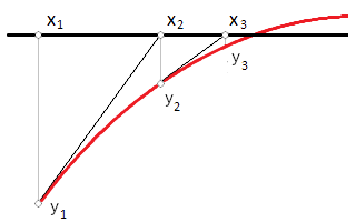
'In the one-dimensional case, we obtain the solution iteratively by constructing the tangent line to the function at the current point and intersecting it with the abscissa to obtain the next point.
'<img style="height:100pt; width:160pt;" src="./Newton.png" alt="Newton.png">
#noc
'This process can be represented by the following equation -'x_ⁿ⁺¹ = x_ⁿ - f(x_ⁿ)/f′(x_ⁿ)
'In the multidimensional case, 'x' is a vector, 'f' is a vector-valued function, and 'f′' is replaced by the matrix of the partial derivatives, called "Jacobian" ('J'). So, the above equation is transformed to the expression:'x_ⁿ⁺¹ = x_ⁿ - J(x_ⁿ)^-1*f(x_ⁿ)', where'J_ij = df_i/dx_j'. The solution is performed as follows:
#equ
'Define the equations as functions:
'  'f_1(x) = 5*x.1 + 4*x.2 + x.3 - x.4^2
'  'f_2(x) = x.1^2 - x.2 + 2*x.3 - sqrt(abs(x.4)) - 3
'  'f_3(x) = 3*x.1^3 - 2*x.2^3 + 3*x.3 + 2*x.4 - 4
'  'f_4(x) = 4*x.1 - 3*x.2 + x.3^2 + x.4 - 11
'Represent the whole system as a single vector-valued function:
'  'f(x) = [f_1(x); f_2(x); f_3(x); f_4(x)]
#noc
'Define the Jacobian matrix containing the partial derivatives of the function'f':
#equ
J(x) = [5; 4; 1; -2*x.4| _
       2*x.1; -1; 2; -1/(2*sqrt(abs(x.4)))| _
       9*x.1^2; -6*x.2^2; 3; 2| _
       4; -3; 2*x.3; 1]
#equ
'Initial guess -'x = [2; 2; 2; 2]
#hide
#for n = 1 : 1000
    x⁰ = x
    δx = inverse(J(x⁰))*f(x⁰)
    ε = norm_e(δx)/norm_e(x)
    #if ε < ε_max
        #break
    #end if
    x = x⁰ - δx
#loop
#show
'Calculate the following expressions iteratively (the last results are displayed only):
'  'x⁰ = x' - store the previous vector <var>x</var>
'  'δx = inverse(J(x⁰))*f(x⁰)'- difference
'  'x = x⁰ - δx'- update the solution vector
'  'ε = norm_e(δx)/norm_e(x)'- relative error
#noc
'Loop until'ε'&lt;'ε_max'or'n'&le;'1000'(guard limit in case of divergence).
#equ
'Completed in'n'iterations at'ε'&lt;'ε_max'.
'Result -'x
'Check -'f(x)
'<h4>3. Broyden’s method</h4>
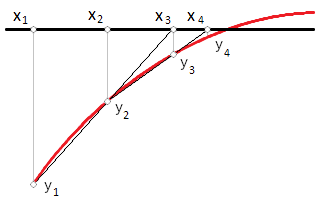
'The Broyden’s method is the mulidimensional equivalent to the secant method. It is similar to Newton’s method, but instead of calculating the inverse Jacobian on each iteration, it uses the secant between two consecutive approximations.
'<img style="height:100pt; width:160pt;" src="./Secant.png" alt="Secant.png">
'Although its convergence is slower, it avoids the heavy operation on computing and inverting the Jacobian each time. The solution is performed as follows:
#equ
'Initial guess -'x⁰ = [2; 2; 2; 2]
'Find the first approximation by using the Jacobian as in Newton-Raphson’s method
y⁰ = f(x⁰)
J_inv = inverse(J(x⁰))
x¹ = x⁰ - J_inv*y⁰
y¹ = f(x¹)
'Correction factor to improve stability -'α = 0.9
#hide
#for n = 1 : 1000
    Δx = x¹ - x⁰
    Δy = y¹ - y⁰
    ΔxT = transp(Δx)
    ΔxTJΔy = ΔxT*J_inv*Δy
    J_inv = J_inv + (Δx - J_inv*Δy)/ΔxTJΔy*ΔxT*J_inv
    δx = J_inv*y¹
    ε = norm_e(δx)/norm_e(x)
    #if ε < ε_max
        #break
    #end if
    x² = x¹ - α*δx
    y² = f(x²)
    x⁰ = x¹','y⁰ = y¹
    x¹ = x²','y¹ = y²
#loop
#show
'Calculate the following expressions iteratively (the last results are displayed only):
'  'y⁰ = f(x⁰)'- function values at prev. step
'  'x¹ = x⁰ - J_inv*y⁰'- current step approximation
'  'y¹ = f(x¹)'- function values at current step
'  'Δx = x¹ - x⁰'- difference in approximations
'  'Δy = y¹ - y⁰'- difference in function values
'  Update the inverse of the Jacobian using the Sherman–Morrison formula:
'  'ΔxTJ_inv = transp(Δx)*J_inv
'  'ΔxTJΔy = ΔxTJ_inv*Δy
'  'J_inv = J_inv + (Δx - J_inv*Δy)/ΔxTJΔy*ΔxTJ_inv
'  'δx = J_inv*y¹'- difference
'  'x⁰ = x¹ - α*δx'- next approximation
'  'ε = norm_e(δx)/norm_e(x)'- relative error
#noc
'Loop until'ε'&lt;'ε_max'or'n'&le;'1000'(guard limit in case of divergence).
#equ
'Completed in'n'iterations at'ε'&lt;'ε_max'.
'Result -'x⁰
'Check -'f(x⁰)

Spotted an error? Edit these examples.